How to migrate a V2 project to V3?

This tutorial will guide you in migrating projects from V2 to V3.

V3 introduces the new SENSE engine by the Sympheny team, enhancing data processing and enabling faster solving for more complex planning scenarios.

Migrate project

Migrating projects from V2 to V3 is easy!

Video Tutorial

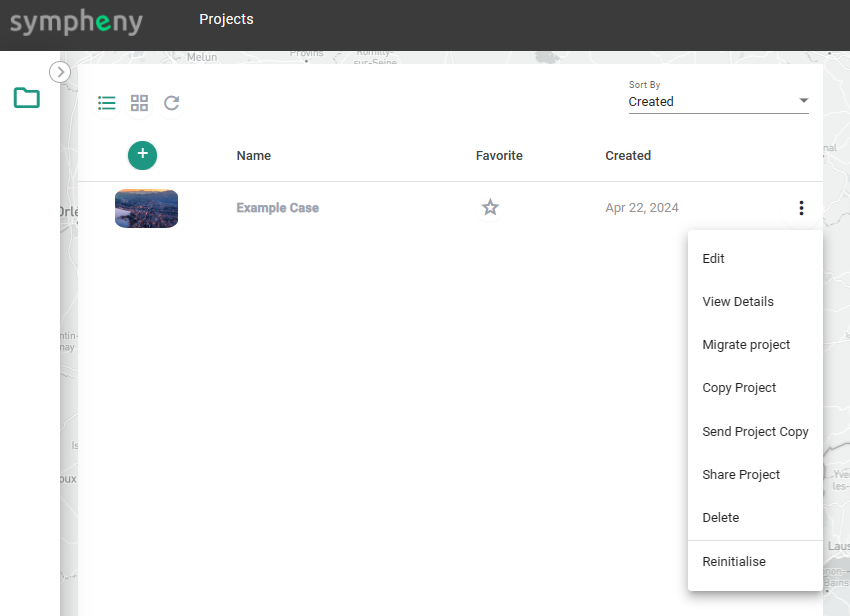
1. Go to the projects navigator page, and click on the three dots icon

2. From the drop down list, click “Migrate project“

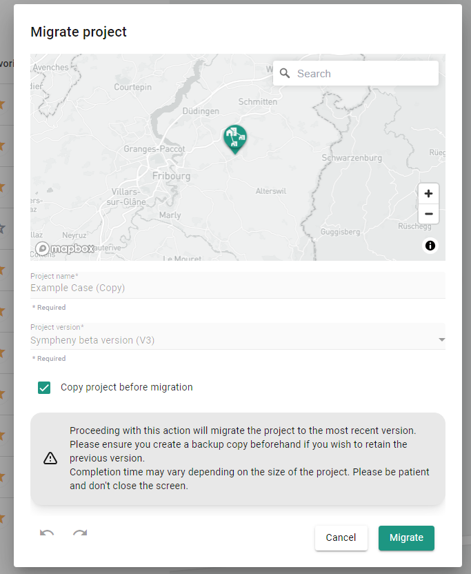
3. Optional (but recommended) - Click “Copy project before migration“ to save a V2 copy for later reference

4. From the pop-up window, click “Migrate“

5. The migrated project in Sympheny V3 is now available on the project page

Review the models

Along with the upgrade to the SENSE engine, we have updated some modelling conventions, with the aim to provide a cohesive modelling framework and more flexibilities in the future.

In case for the migrated projects, all of the boundary conditions are retained (Steps 1, 2, 3, 4 and 6), we recommend the user to review the models in Steps 5 and 7.

General (Step 1)

Stages

The introduction of stages within V3 is one of the key feature, as it allows users to model multiple stage models. The stage feature has an influence on the calculation of the financial objective, when considering multi-stages.

Note: When migrating from V2 to V3, a stage is generated with a length equal to the maximum lifetime of the technologies in V2. Consequently, this should not affect the results.

On-site Resources (Step 5)

V2: Rated vs. Nominal Capacity

In V2, users specify whether the technologies connected to on-site resources (with hourly resource availability profiles), are designed with rated or nominal capacities.

In the case of rated capacity, the kWp of the technologies is calculated based on standard values (e.g., 1kW/m2 for the case of PV). The kWp value is the one relevant for the technology sizing and investment costs.

In the case of the nominal capacity, the maximum output capacity in kW that could be achieved according to the hourly profile is used to determine the sizing of the technology, relevant for the costs.

Example: Solar Panels

Imagine you install 250 kWp of solar panels on a roof (rated capacity based on standard conditions). However, the location's maximum irradiation reaches 1.1 kW/m². Therefore, the 250 kWp system can potentially output 275 kW whenever irradiation reaches 1.1 kW/m².

V3: Peak Power Parameter

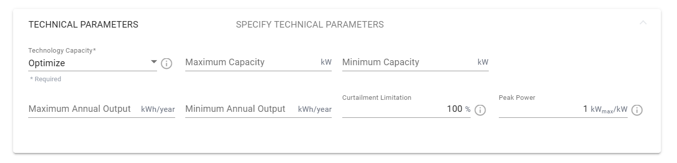
In V3, the nominal or rated consideration is not specified at the on-site resources step, but directly linked to the conversion technology candidates. In the technical parameters, you can specify the Peak Power parameter, in order to set your preferred sizing principle. This streamlined approach for defining renewable technology capacity allows users to select the method that best suits your requirements, while connecting the same on-site resources across multiple technologies.

• Nominal capacity: Set the Peak Power parameter to 1 kW_max / kW. This means the PV panels sizing is the peak power of the panels, and the investment cost is calculated base on this value.

• Rated capacity: Set the Peak Power parameter to max(Irradiation Profile) / standard value kW. This means for the 250 kWp installation example, that the Peak Power needs to be 1.1/1 = 1.1. This mean that to produce the 1.1 kW/m2, ‘only’ 1 kWp will need to be installed and paid for.

Tip: You can find the max value of the profile by viewing the profile in the on-site resource step.

Exports (Step 6)

This section explains how export pricing works differently in V2 and V3. Understanding these changes are important for a smooth migration from V2 to V3.

• V2: In the older version, Capacity Sale Price, in $/kW/year or $/kW/month, is simply considered a cost.

• V3: The new version offers more flexibility. Prices for both Import and Export Candidates can be positive or negative, indicating either a cost incurred or revenue generated.

Key adjustment after migration:

For Export Candidates in V3, positive values indicate revenue earned, while negative values indicate cost incurred.

Therefore, during the migration from V2 to V3, Capacity Prices for Export Candidates are adjusted to negative values to maintain consistency with V2, in which the parameters represent costs.

Conversion Technologies (Step 7)

Technology Modes

The Technology Modes are undergoing a consequent change in the modelling conventions. In V3, the output efficiencies are calculated based on the total input energy, while in V2, it’s only based on the primary input. There is no more setting on “primary input” in V3.

This allow users to gain a clearer understanding of energy dissipation within their systems. The sum of the output efficiencies now directly reflects the system's total efficiency. Specifically:

• If the total efficiency equals 100%, it indicates that useful energy is conserved within the system.

• If the total efficiency is less than 100%, it suggests that useful energy is lost in the system.

• If the total efficiency exceeds 100%, it implies that useful energy is created within the system.

In V2, a 100% output efficiency did not necessarily mean that useful energy was conserved, as it only referred to the primary energy input. This approach allows for a clear separation between behaviors related to input shares and those related to efficiencies. In V2, COP (Coefficient of Performance) information had to be entered both in the input shares and in the output efficiencies. However, in V3, the COP can be defined solely within the input shares, while the output efficiencies can focus on specifying any mechanical losses of the heat pump.

This change also simplifies the integration of hourly parameters for input shares that may differ from output efficiencies. As a result, users no longer need to set a "variable input ratio" for multi-input technologies when dealing with time-varying efficiencies, as this is now automatically managed by the new modeling convention.

Example 1 - Heat Pump

For instance, a heat pump with a COP of 3 is defined as such:

Calculation:

• In V2:

Output i = Primary Input * Efficiency Output i

HT Heat = 100 * 300% = 300

In this case, 100 units of Electricity will lead to 300 units of HT Heat. No matter what is the input share of Ambient Heat.

• In V3:

Output i = Sum of Inputs * Efficiency Output,

HT Heat = (100 + 200) * 100% = 300

In this case, 100 units of Electricity and 200 units of Ambient Heat will lead to 300 units of HT Heat.

In order to correctly model the behavior of the technologies, the output efficiencies are recalculated using this equation:

V3 Output Efficiency = (Primary Input Share * V2 Output Efficiency) / Sum of input shares.

For the heat pump example, it leads to:

V3 Output efficiency of HT Heat = (100 * 300%) / 300 = 100%

Note: When migrating a project from V2 to V3 and for fixed efficiencies, this recalculation is automated using the provided equation. Therefore, manual recalculation of output efficiencies is unnecessary.
If you have technologies containing hourly or monthly efficiencies, these have to be adapted manually.

Example 2 - Chiller

This section is for information only. Chillers are migrated from V2 to V3 without need for user verification.

For chillers, there are two ways to model Cooling Energy. The first method assumes Cooling Energy as a service, meaning the energy is generated and supplied. This was the default approach in V2 and will remain the same in V3 just after migration. For example, when modeling a chiller with an Energy Efficiency Ratio (EER) of 2, the process would be as follows:

This means that an input of 100 units of electricity will result in the generation of 200 units of cooling (based on an EER of 2) and 300 units of heating (assuming the electricity is fully dissipated as heat). This approach is similar to the construction used in V2.

However, in V3, there is an alternative method where Cooling Energy is treated as an extraction of energy demand. To use this method, you should set the Cooling Demand to "reversed." In this case, the chiller can be modeled as a heat pump with an EER of 2 (or COP of 3).

E-Mobility Parameters - Storage Technology Candidates

• V2: EVs could be modelled as storage technology candidates by activating the E-MOBILITY PARAMETERS (see documentation: Add EV Batteries).

• V3 (V3.4): In the current version (V3.4), the E-MOBILITY PARAMETERS are not not yet available. We plan to re-introduce these parameters in the V3.5 release (Q1 2025). Meanwhile, users could model EVs with the alternative method (see documentation: Add EV Batteries | 4.-Can-I-model-EV-as-a-demand-instead?).

During migration from V2 to V3, this is one of the few steps that requires manual migration. Here are the steps:

1. From the V2 Output files, download mobility profiles. Navigate toResult Tables\ScenarioName_Point #.xlsx. Open the excel sheet named after the storage technology candidate that contains E-MOBILITY PARAMETERS, and extract the “Flow Charge(kWh)“ column to obtain the energy demand profile (TEMPLATE PROFILE XLSX).

2. In the migrated V3 scenario, upload e-mobility profiles as energy demands.

3. In the migrated V3 scenario, delete the storage technology candidate containing the E-MOBILITY PARAMETERS.

Objective Function & Results

This section covers how to achieve the same results in V3 as your single-stage V2 projects.

Matching V2's Objective Function:

• In V3, select "Minimum Annualized Life-Cycle Cost" to mirror the objective function used in V2. V3 provides additional options, but you can find detailed explanations in the full Sympheny V3 documentation.

Understanding Cost Presentation:

• V2 projects displayed life-cycle costs as EAC (Equivalent Annualized Cost). In V3, these costs are presented as NPC (Net Present Cost).

• You can still access the EAC values in the exported Excel sheets.

Note: In single-stage models, the following objectives have the same outcome:

• Minimum Life-Cycle Cost

• Minimum Annualized Life-Cycle Cost

NPC and EAC

NPC calculates the present value of all cash flows across years, considering the time value of money. EAC converts the cost of investments with different lifespans or cash flow patterns into equal annual payments.

For the migrated projects in V3, users can expect that the EAC will remain consistent with what was seen in V2. There could be a slight variation (up to 5%) due to the difference in time resolution or optimization parameters (e.g. optimality gap) set by the user in V3. If this is not the case, please send your questions (see next session).

The NPC representing the discounted sum of cash flows across all years per stage. This includes all costs and revenues for all components in the model.

To determine the EAC, begin by calculating the CRF (Capital Recovery Factor):

Where i is the real discount rate, and n is the number of years in a stage.

The real discount rate, i, can be calculated using the following:

Finally, the EAC are calculated using the following:

More questions regarding your specific model?

We will be happy to provide migration guidelines for a specific technology model that is not covered in this tutorial. Simply send your questions to our support team via our Help Center or email (support@sympheny.com) or schedule a call to check your models together!

Send a ticket to Sympheny Help Center

1. Head to the Help Center

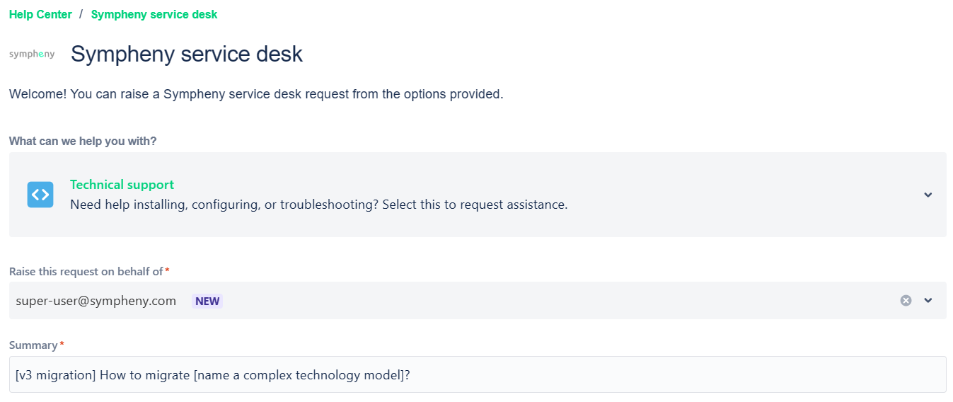
2. Create a ticket by clicking “Technical Support“

3. In the ticket, provide your Sympheny account (email), and fill in the details.

   • In the “Summary” field, please follow this template: [v3 migration] How to migrate [name of your technology]?

   • In the “Description“ field, please provide a description of the technology, and a screenshot of the parameters of your technology in Sympheny V2.

Schedule a call

If you have more than one models in question, or would like to learn more about Sympheny V3, it’s time to hop on a call with the Sympheny support team! Simply pick your preferred slot here.