In this example, we simulate a Data Center. The goal is to help users through their first steps in the Sympheny web app with the mandatory and some optional features. In the following steps we:
-
Create a scenario to size a solar PV installation
-
Evaluate the cost and performance of a 100 kWh battery
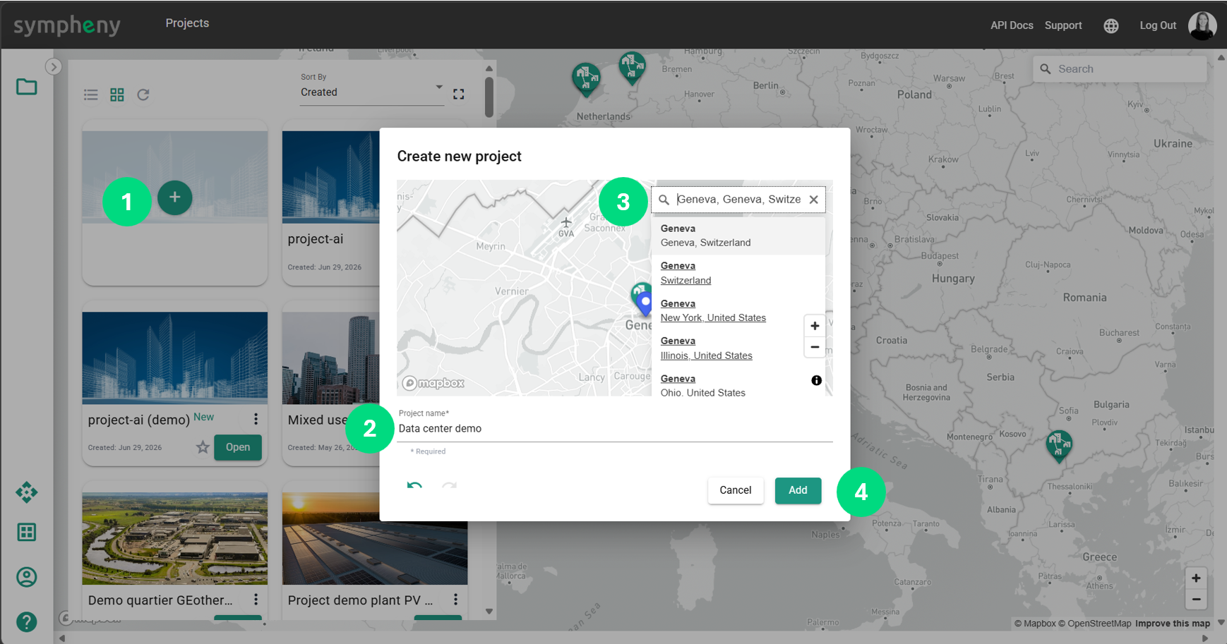
Create a project
The location can be specified by searching for an address.
Create a scenario
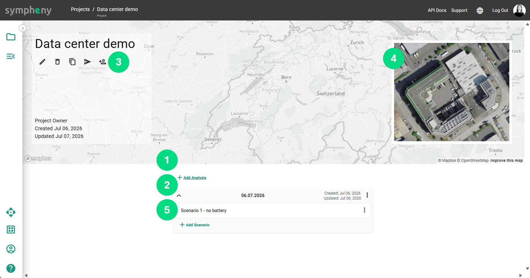
Analysis can be used as archive. Different scenarios can be created to be compared. Then click a scenario to work with it.
-
Send a copy or share the project with other Sympheny users.
-
Upload an image to illustrate your project, with a small resolution
General
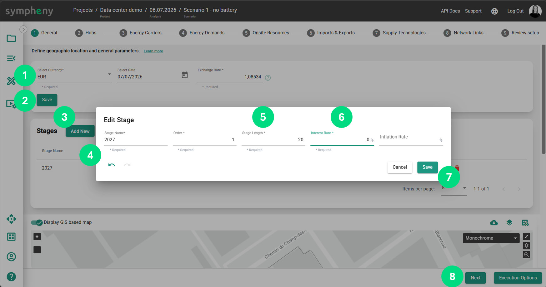
Currency can be changed, press Save after changing currency. Add a stage, multiple stages can be used to plan an optimal energy system over decades although this adds complexity to the modeling process. To get started on a project, simulate a single stage. An interest rate of 0% will help new users interpret the results.
Hubs
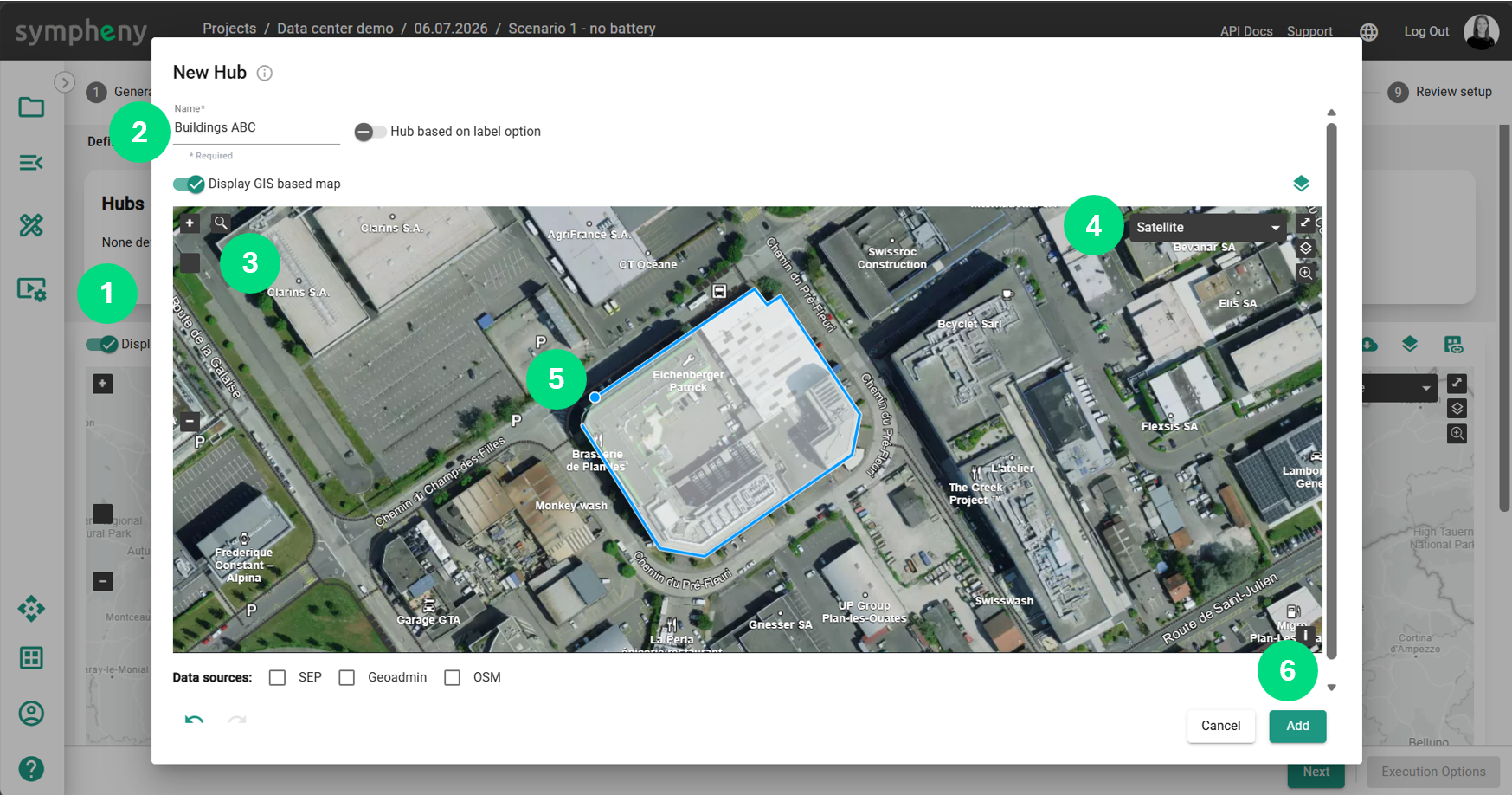
Add new Hub, multiple hubs are used to energy simulate networks like district heating for example. More hubs adds complexity, to get started we simulate a single hub.
-
Location can be researched by address
-
Map overlay can be changed
-
Draw an outline of the building or group of buildings to illustrate and locate them. Addons for extracting geodata from the map can be activated.
We can skip ahead to Supply Technologies where Energy Carriers will be defined automatically.
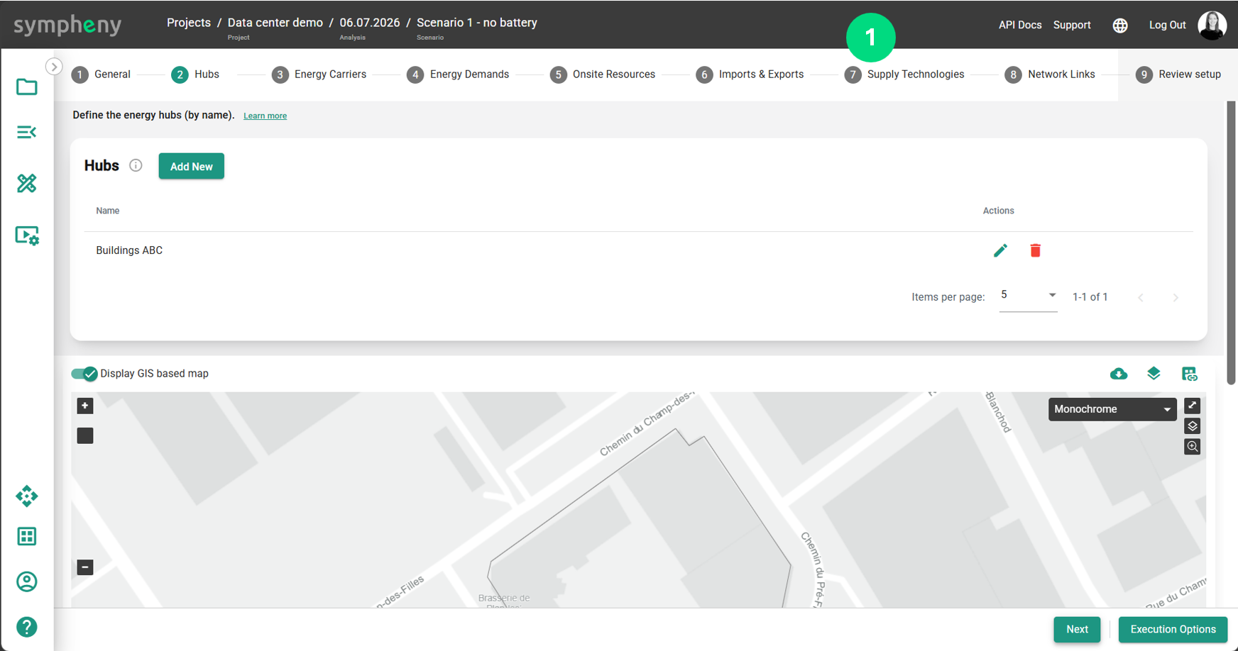
Supply Technologies
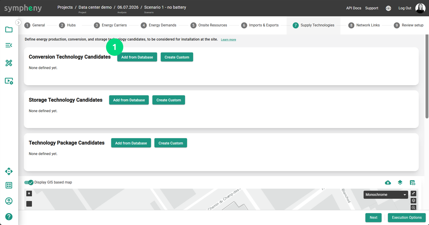
Add a technology from the database.
We select a large solar field, the price per kW will be lower. Once selected, information on the source is available.
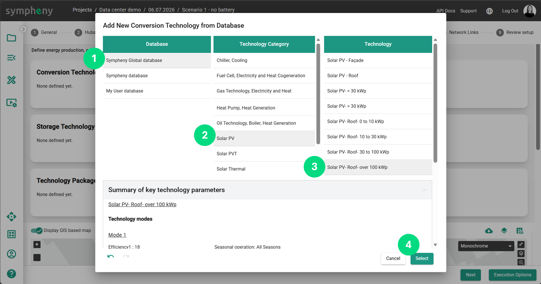
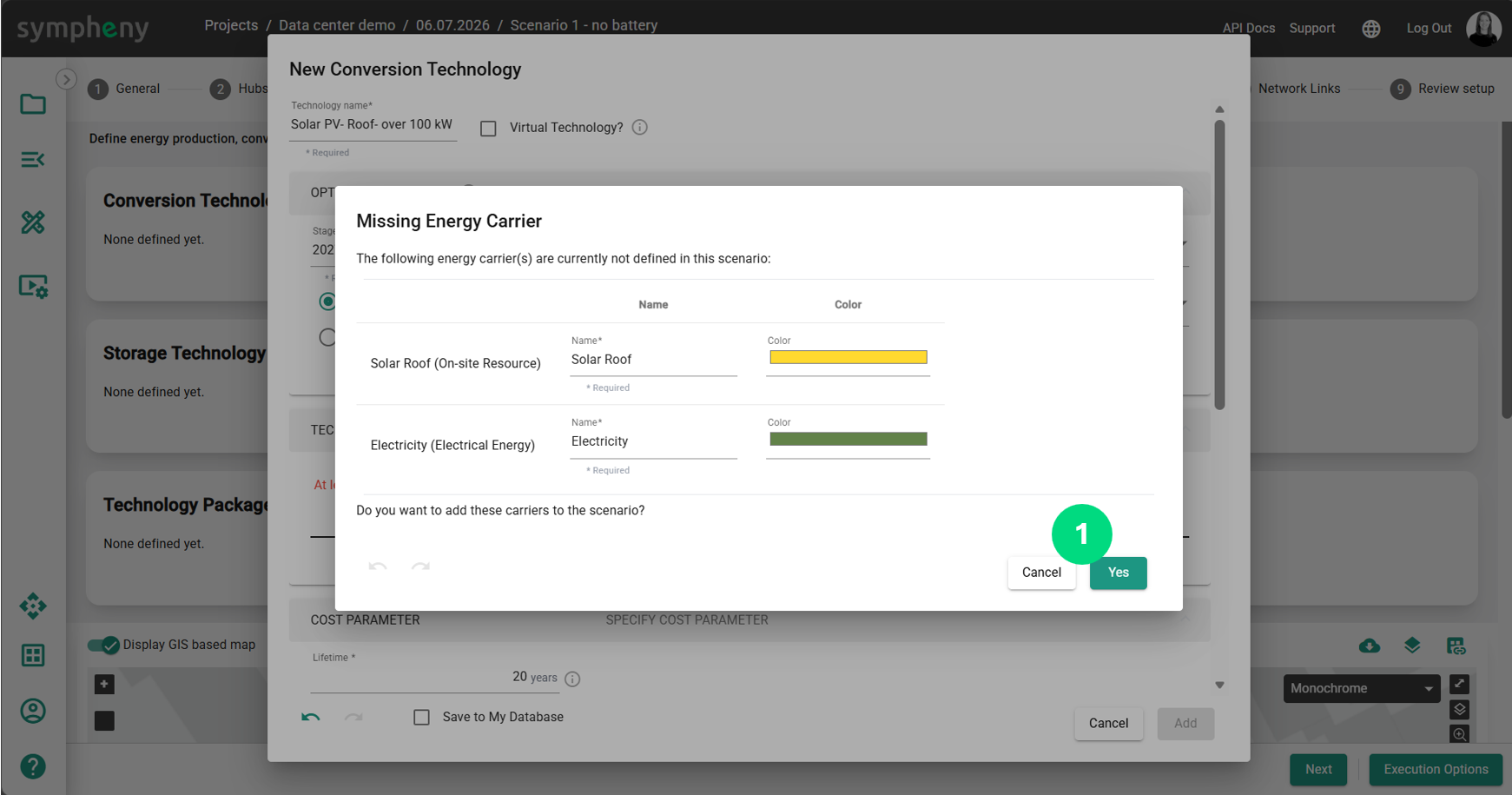
Click Yes to add the energy carriers.
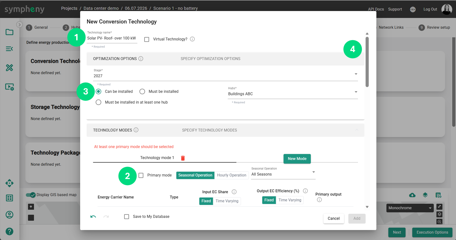
All of the parameters of a technology from the database can be edited. Check Primary Mode every technology needs at least one primary mode. Multi-mode technologies can for example represent a reversible heatpump.
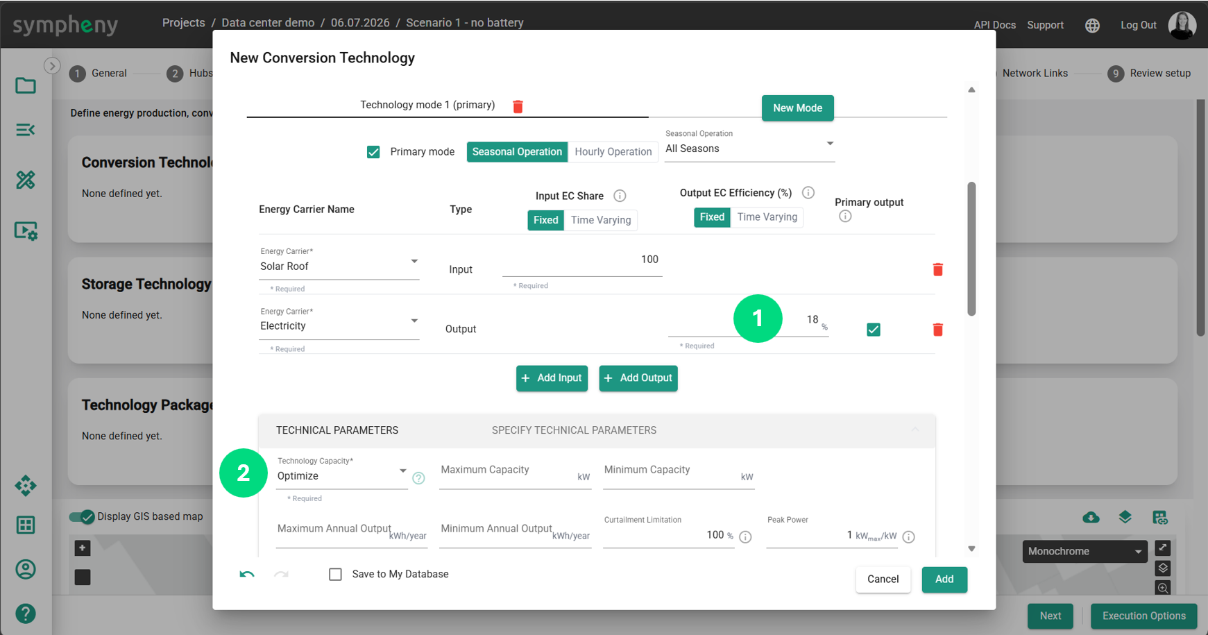
The efficiency of this default solar PV is 18% relative to the solar irradiance caught by the panels. We leave the sizing as Optimize where Sympheny will fix the optimal size to reach the objective, usually minimum ROI.
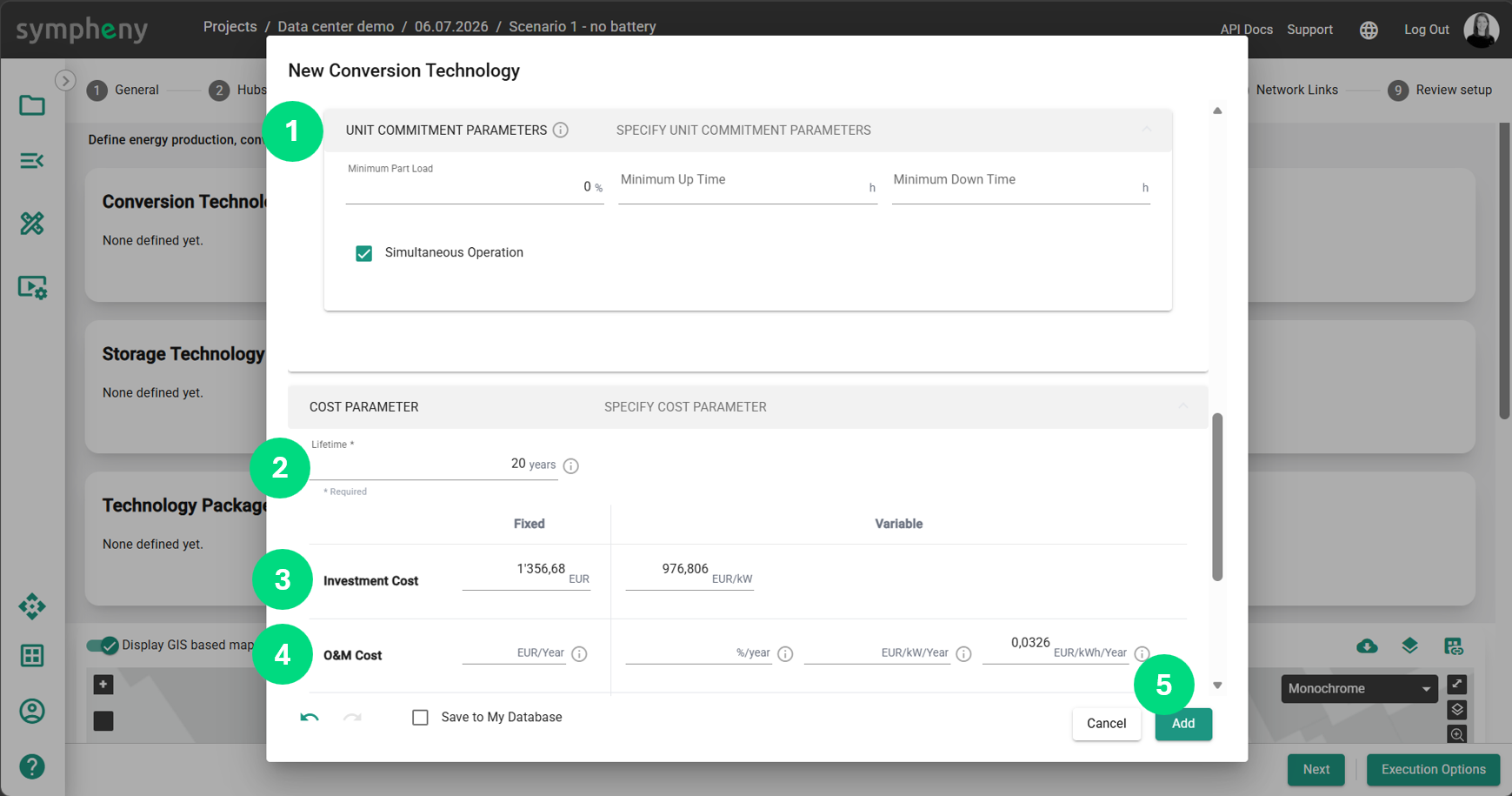
Unit commitment parameters are advanced parameters used for specific industrial equipment's. Parameters related to investment cost, maintenance and embedded emissions can be edited.
Now that the technologies and associated energy carriers are created, we head back to the Energy Carriers step.
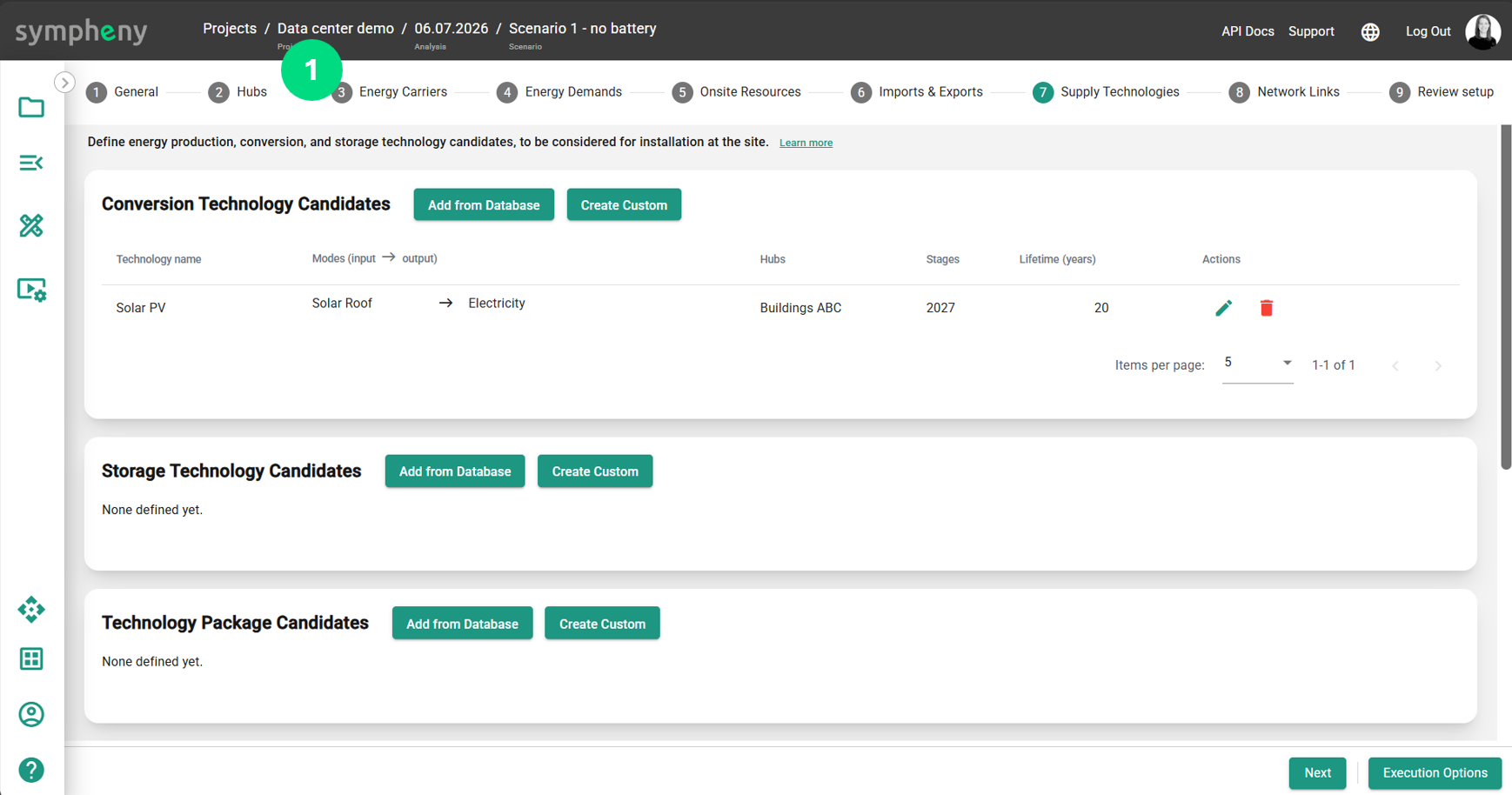
Energy Carriers
It is possible to edit or create more energy carriers to distinguish all of the different energy flows. We use the defaults for this example.
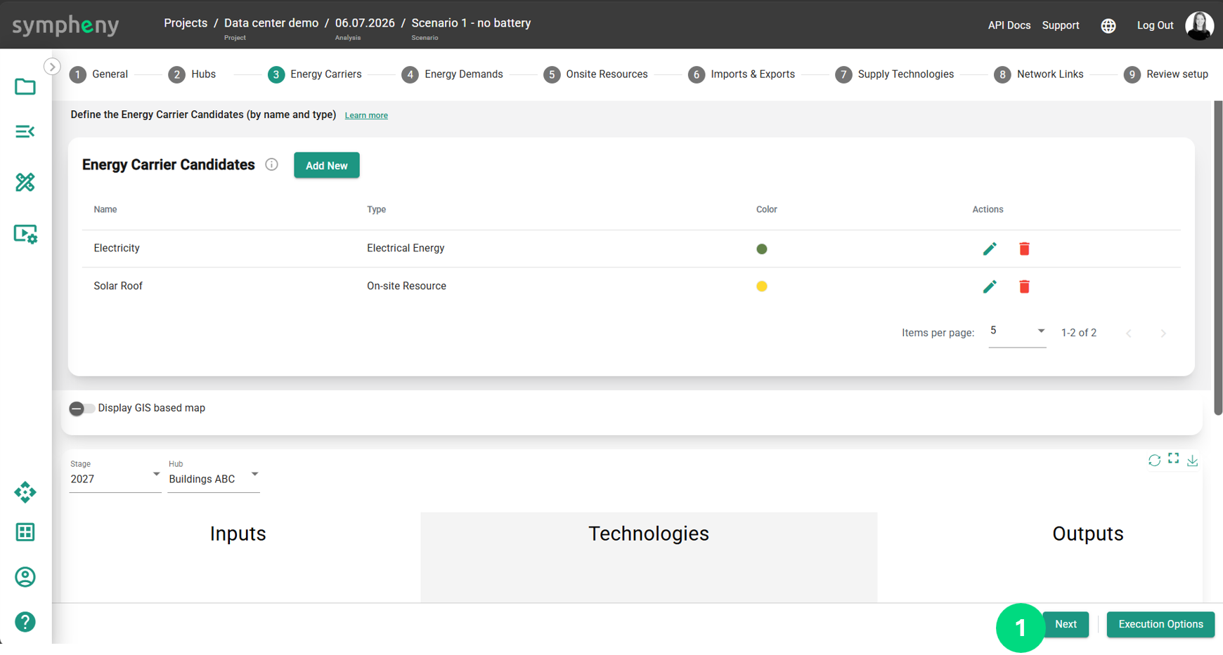
Energy Demands
In all sections we have a map view to represent hubs and networks. Let’s close it to view the technology diagram below. This diagram is dynamic, for now, only the solar panels appear.
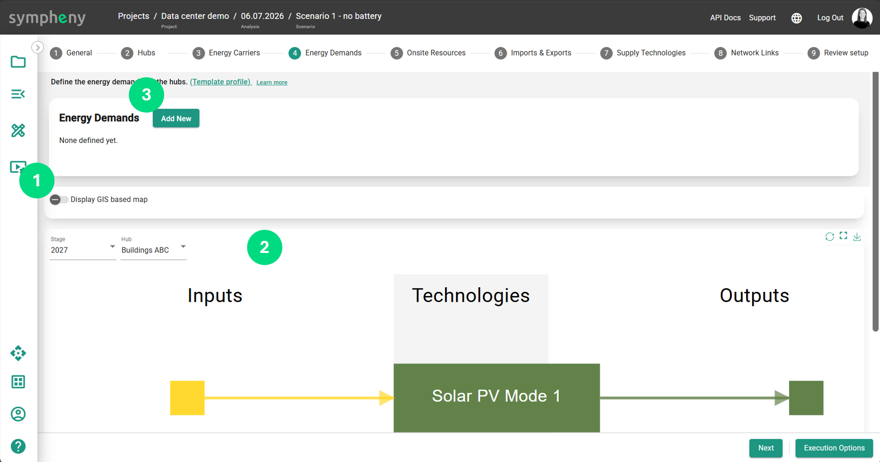
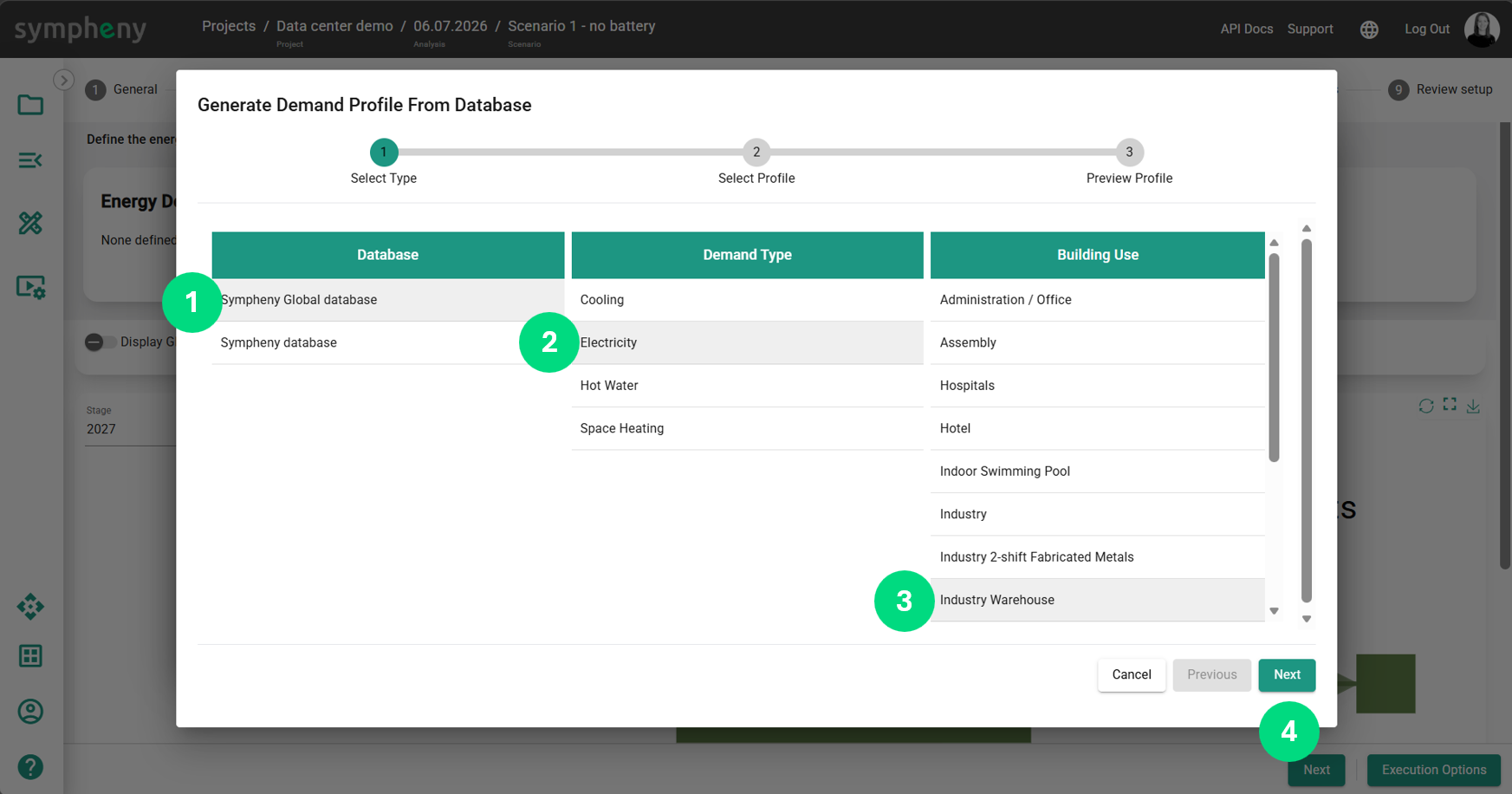
Create a new Energy Demand. Select the energy carrier, the name can be edited. Let’s try to generate a profile for a datacenter using the available profiles.
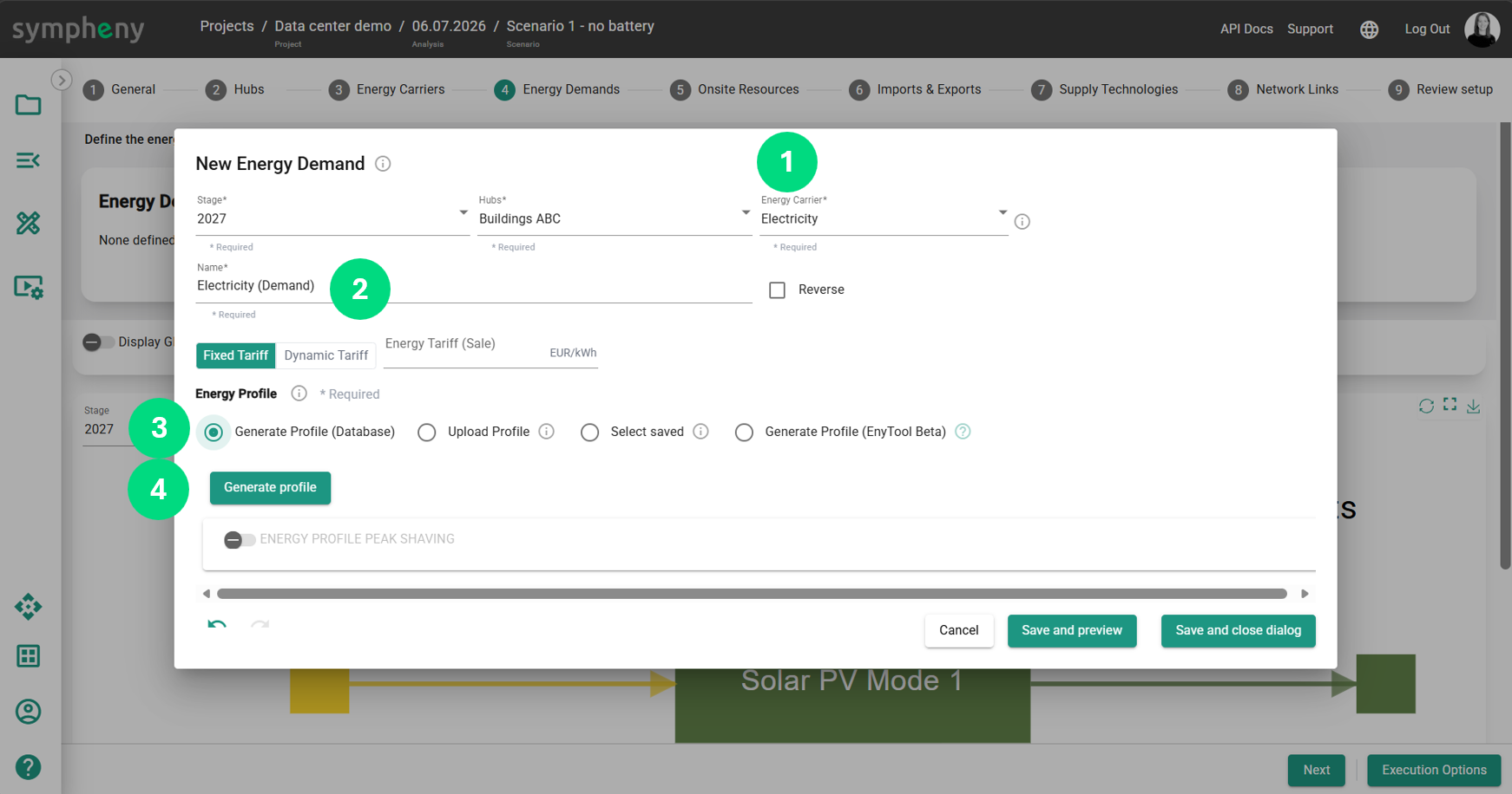
Even if there is no profile called “datacenter” we can explore the available building profiles and see if Industry Wearhouse fits the project needs.
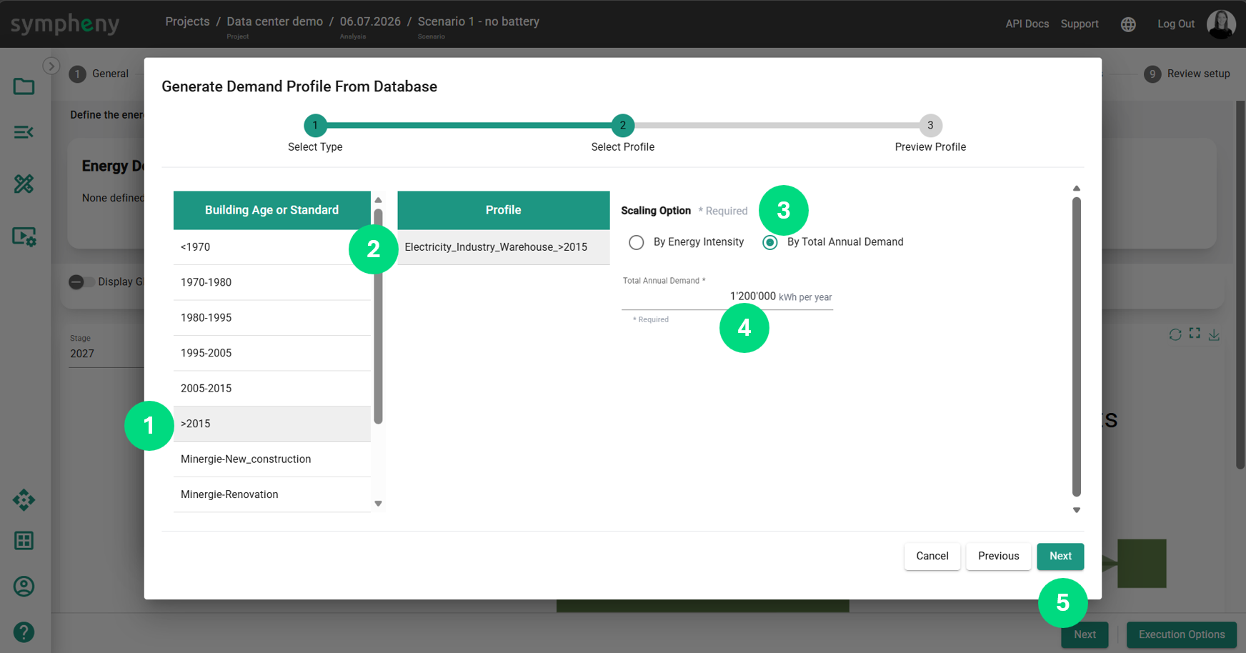
In this case, we have the annual electricity consumption, and can specify 1.2 GWh/year.
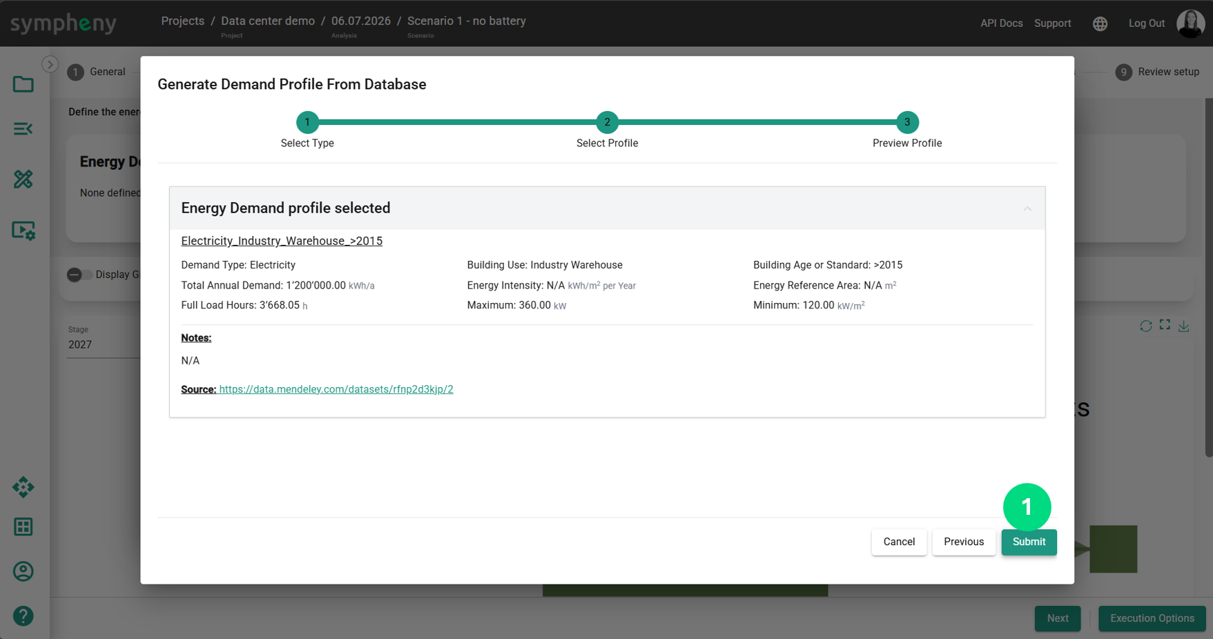
Information on the source of the profile is displayed.
Save and close to add the profile.
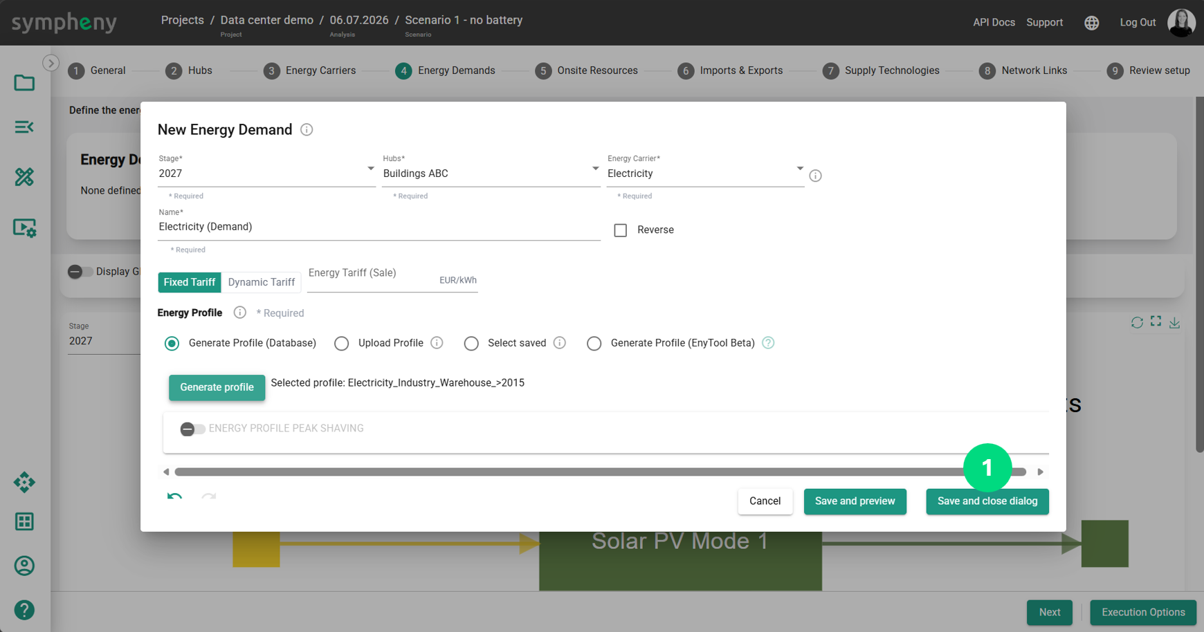
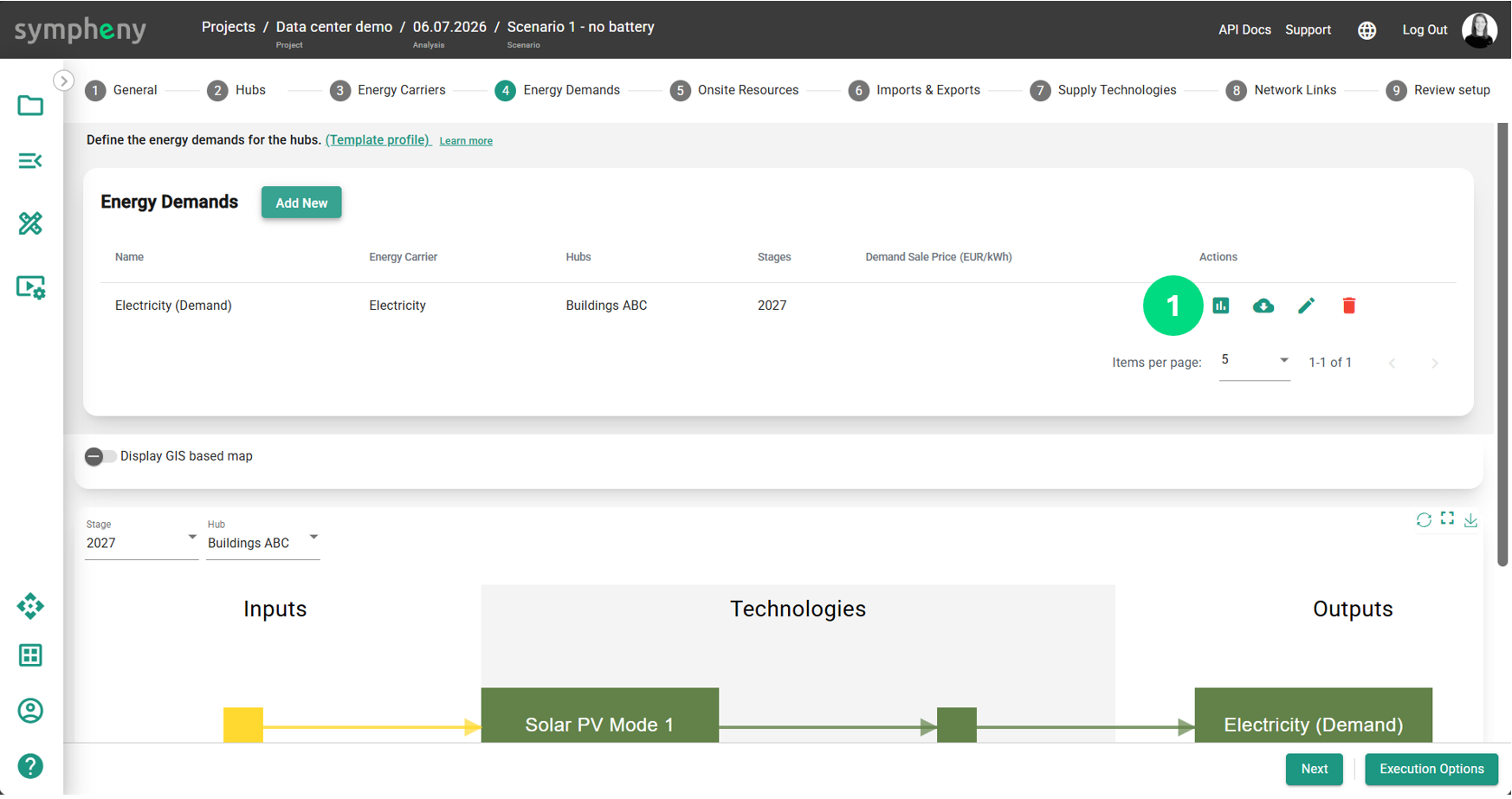
This button allows us to view the profile we generated.
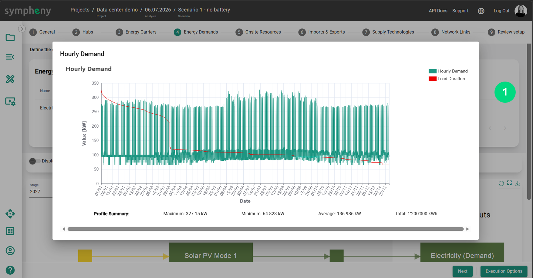
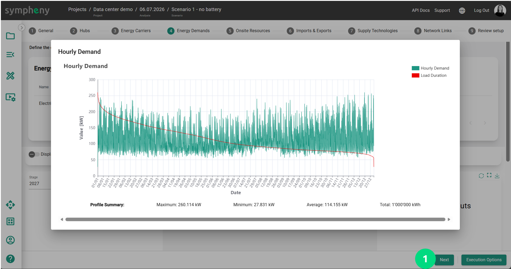
This is the resulting hourly profile. We can see large drops in consumption over weekends. It is possible to download and edit the profile and reupload it. It is also possible to use the Sympheny peak shaving function.
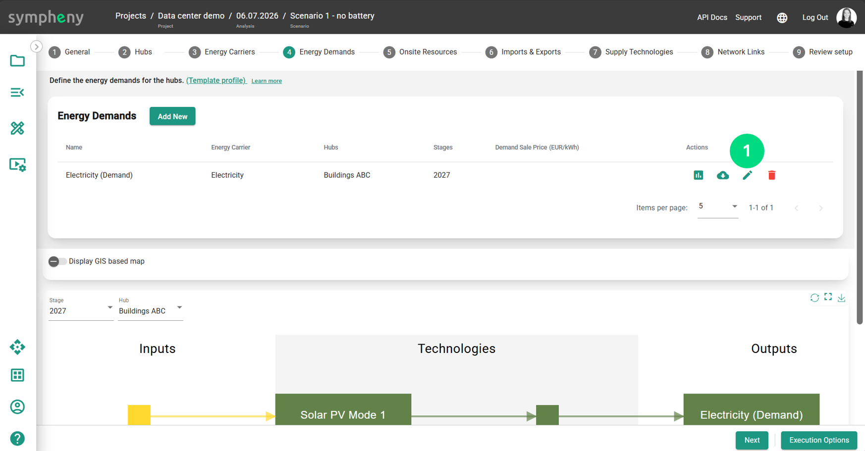
Let’s upload a custom profile. Edit the energy demand.
Select upload profile. The info button describes the format. Downloading the profile will also reveal the format template.
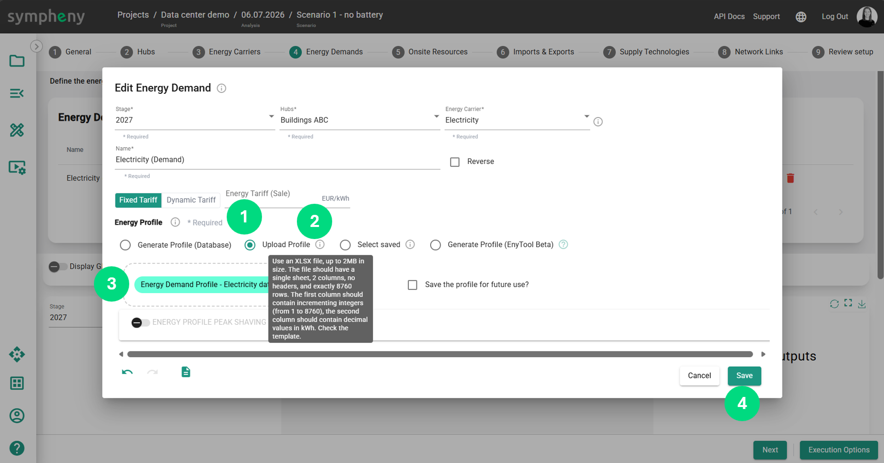
Here is an example of an hourly profile, an excel file with 8760 values in kW.
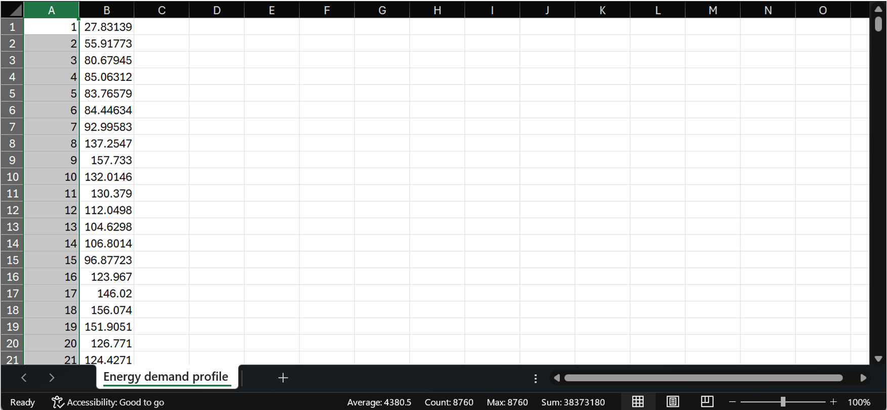
The new uploaded profile has a better shape to represent the electricity demand of a datacenter.
Onsite Resources
In this section we will generate the hourly profile of irradiance hitting the solar panels.
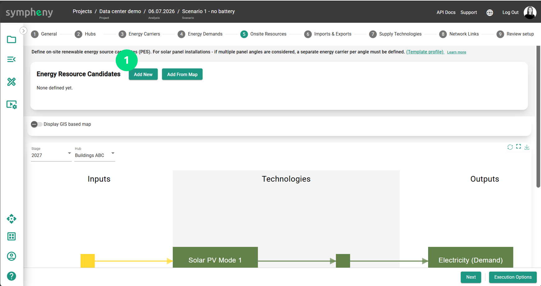
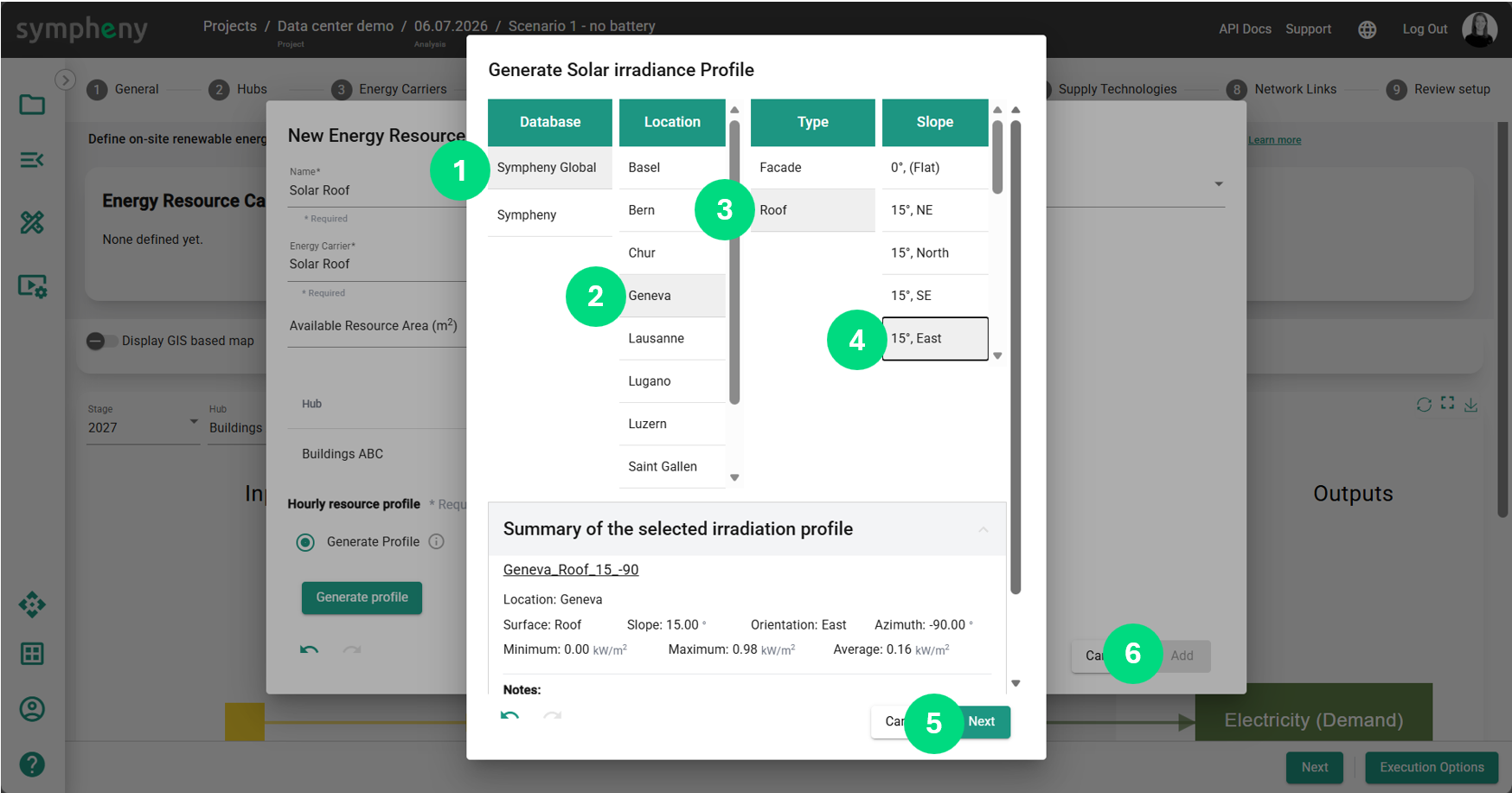
Select the energy carrier, then name can be edited. We set 10’000m2 of available surface of solar panels. And generate the demand based on a location-inclination-orientation available in the database. This represents the maximum available surface. Sympheny will choose the optimal size relative to the electricity consumption, price and resale value.
It is possible to generate the hourly solar profile for any location-orienation-inclination combination using the Add From Map workflow.
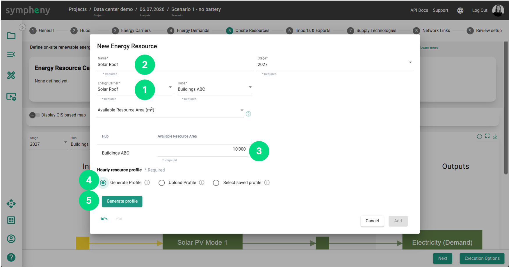
We select Geneva, Roof and 15° East for this solar array.
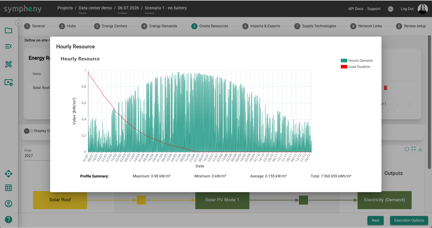
This is the resulting hourly solar irradiance profile, per m2.
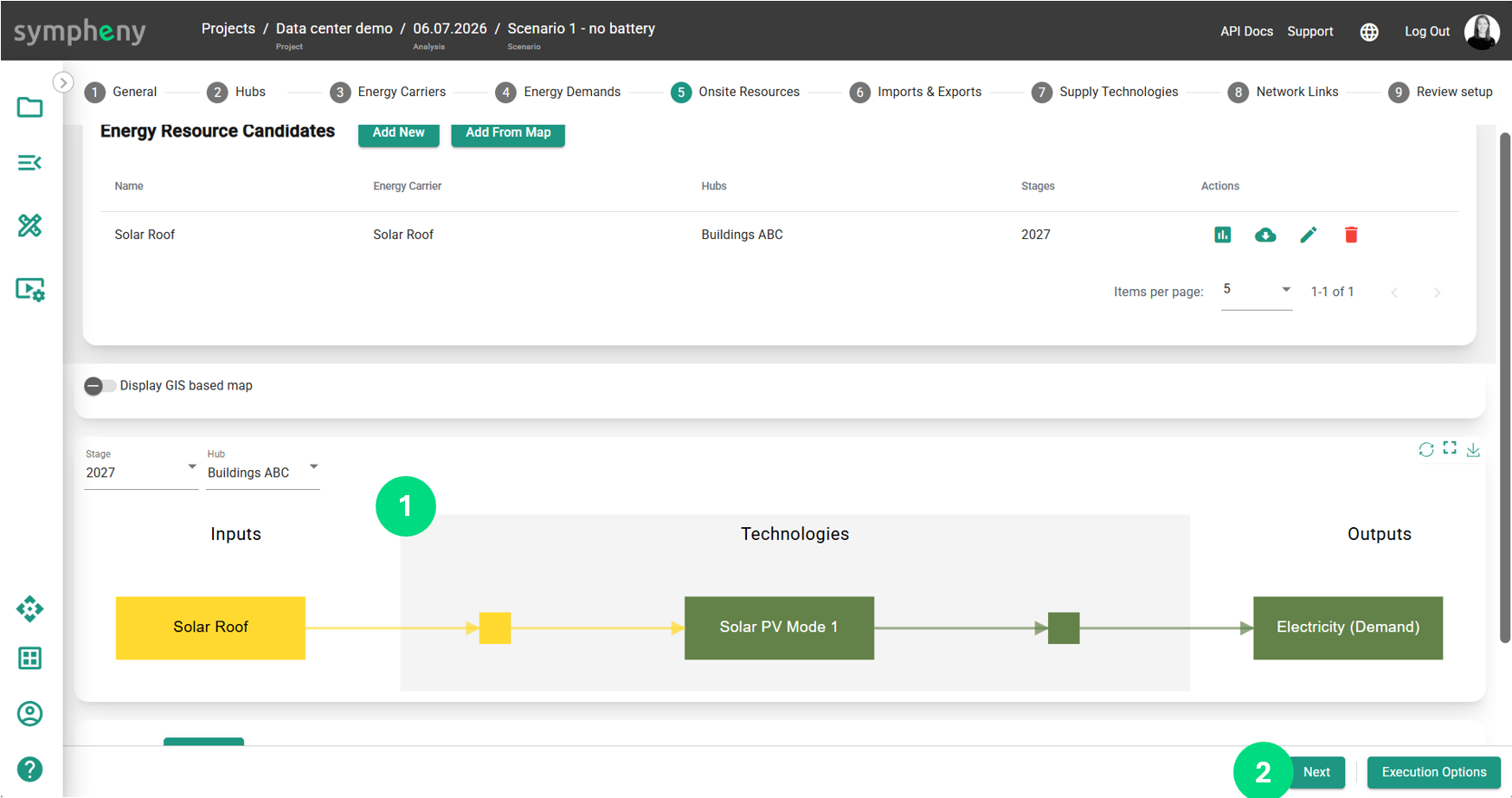
We can see that the Energy Diagram has been updated.
Import & Export
We still need to add the electric grid, otherwise there will be a deficit of electricity during the night and a surplus of electricity during the day may limit the size of the solar field.
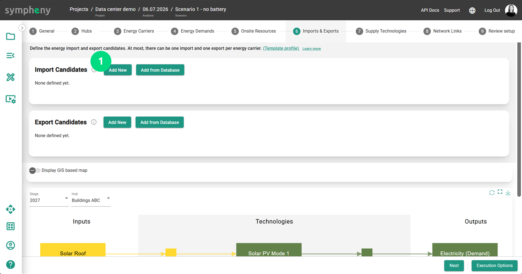
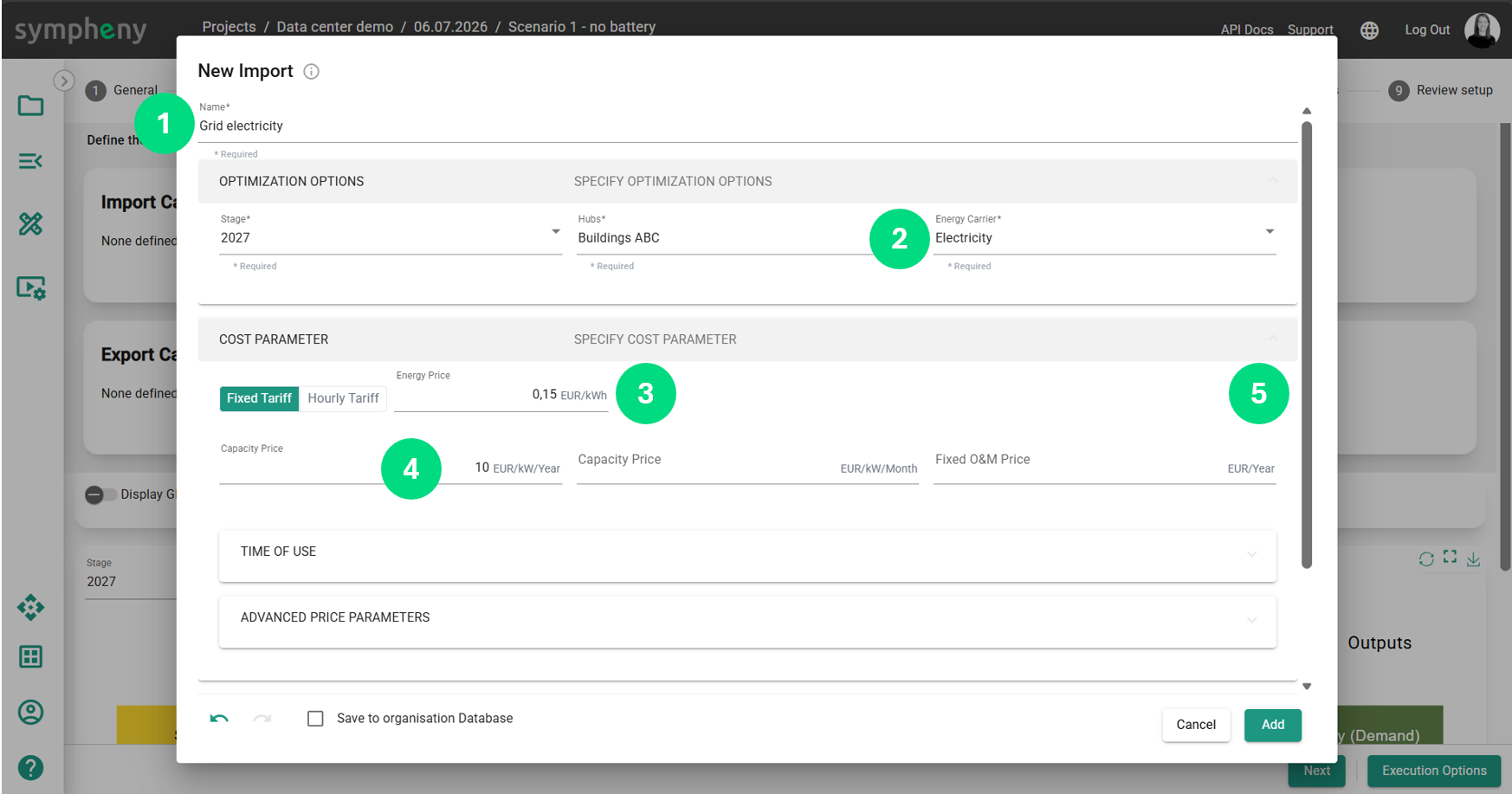
We add the possibility to purchase electricity from the grid. We add the price of electricity.
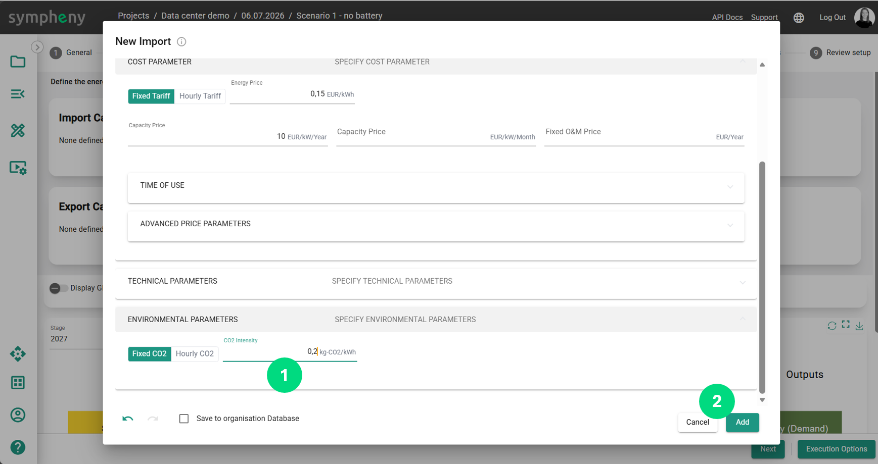
It is optional but best practice to add a capacity price and a value for CO2 emissions per kWh.
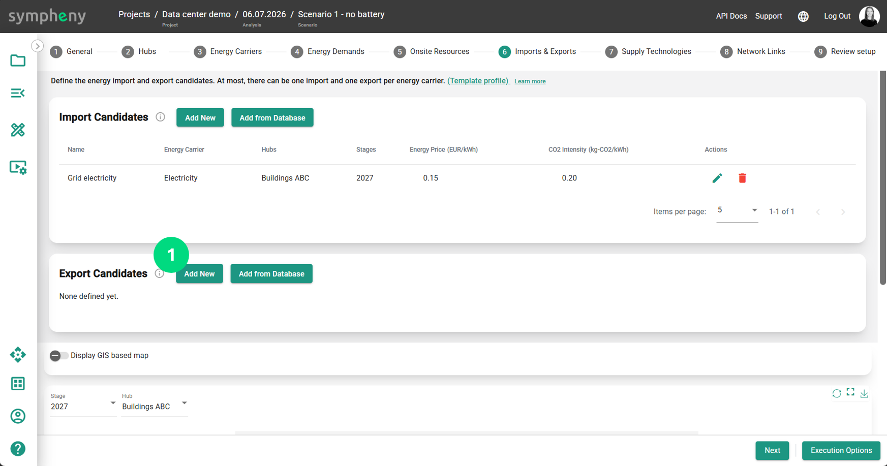
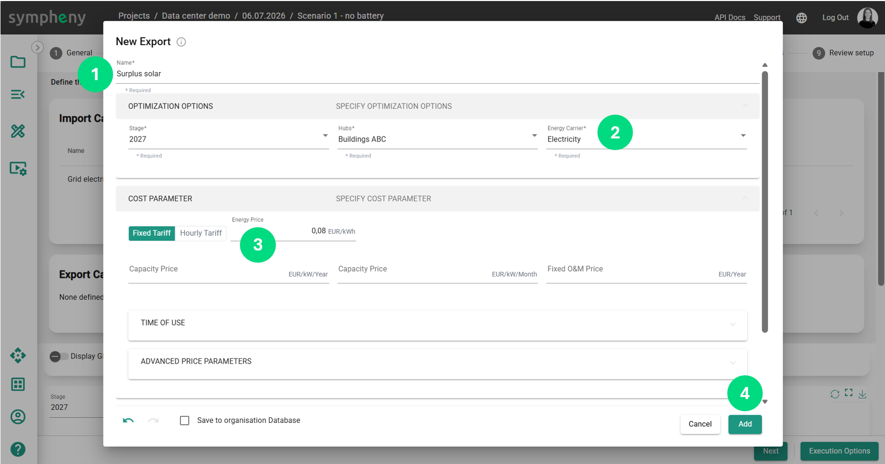
We also add an export, with a revenue value of 0.08 EUR/kWh.
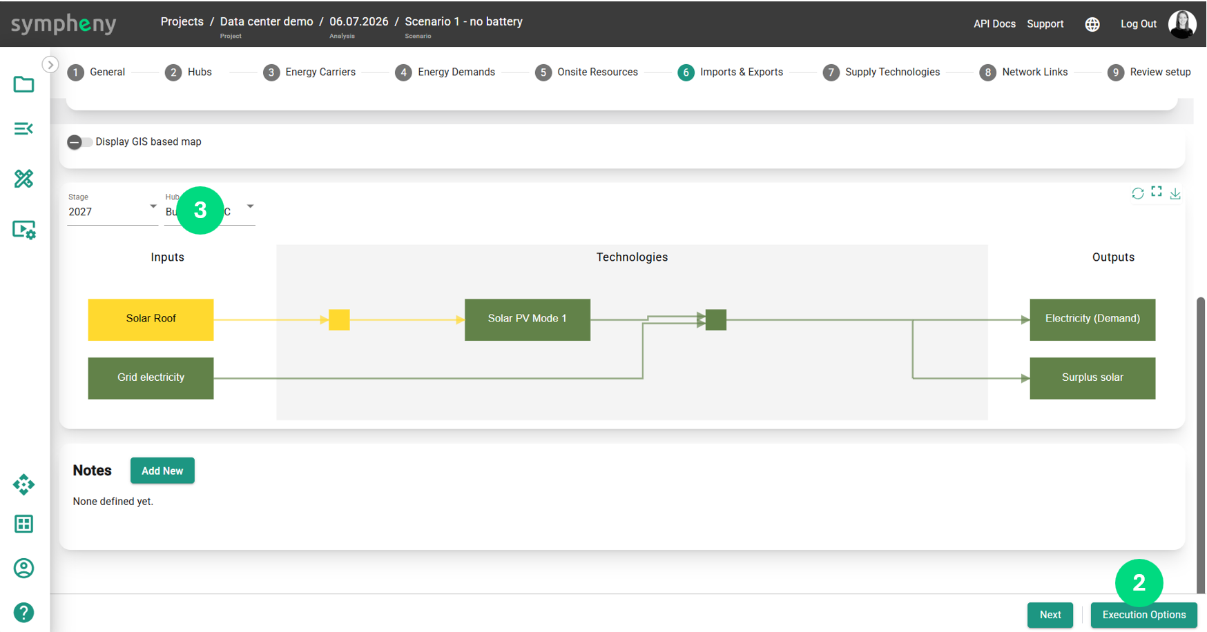
Before executing the model, it is important to view the Energy Diagram. We see that all of the technologies and links are fully connected, there is no dead-end.
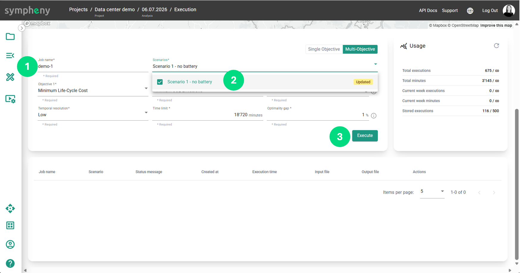
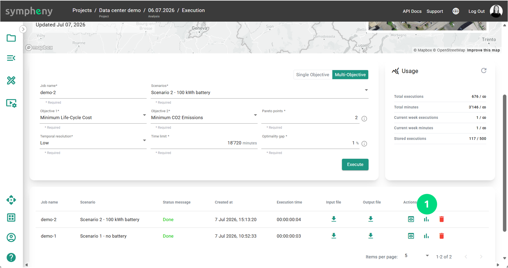
We give a name to the execution. The “Updated” indicator means the scenario has been edited since it was last executed. By default, it generates two solutions. Solution 1 minimizes the total costs = operating costs + maintenance costs + annualized investment costs. Solution 2 minimizes the CO2 emissions.
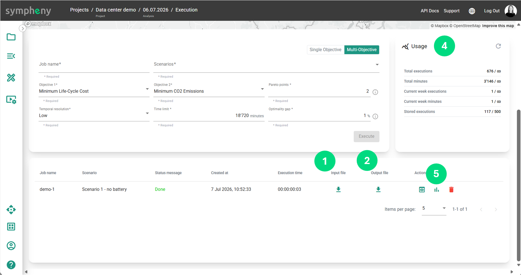
Executing the model takes a few seconds. We open the interactive dashboard to review the results.
It is possible to explore the input file, with all parameters and the output files with all of the results. These are Excel files.
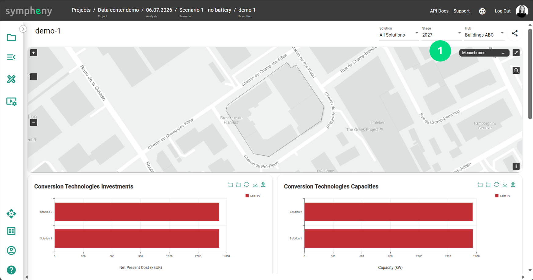
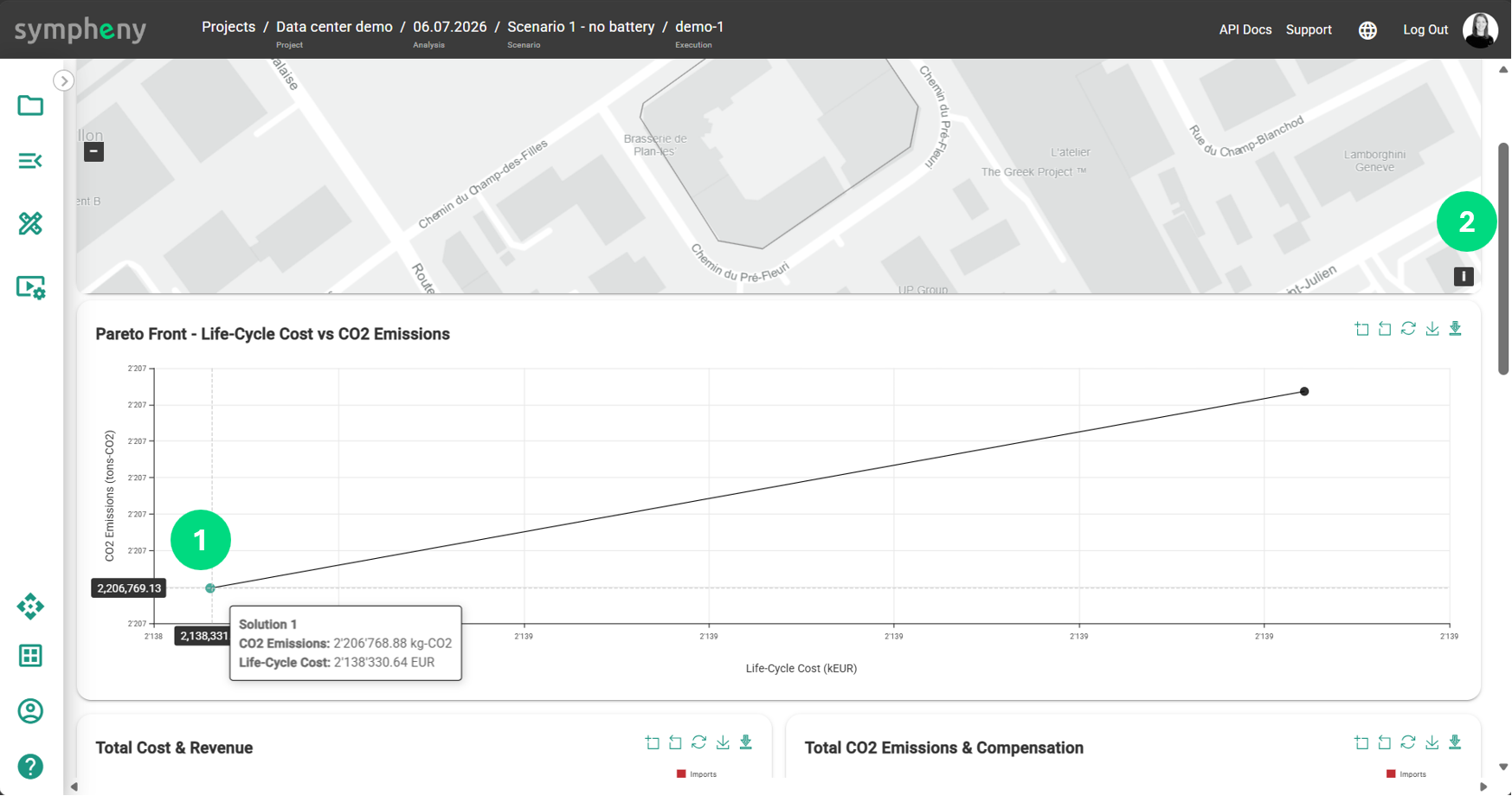
First, we select All Stages to view the Pareto front.
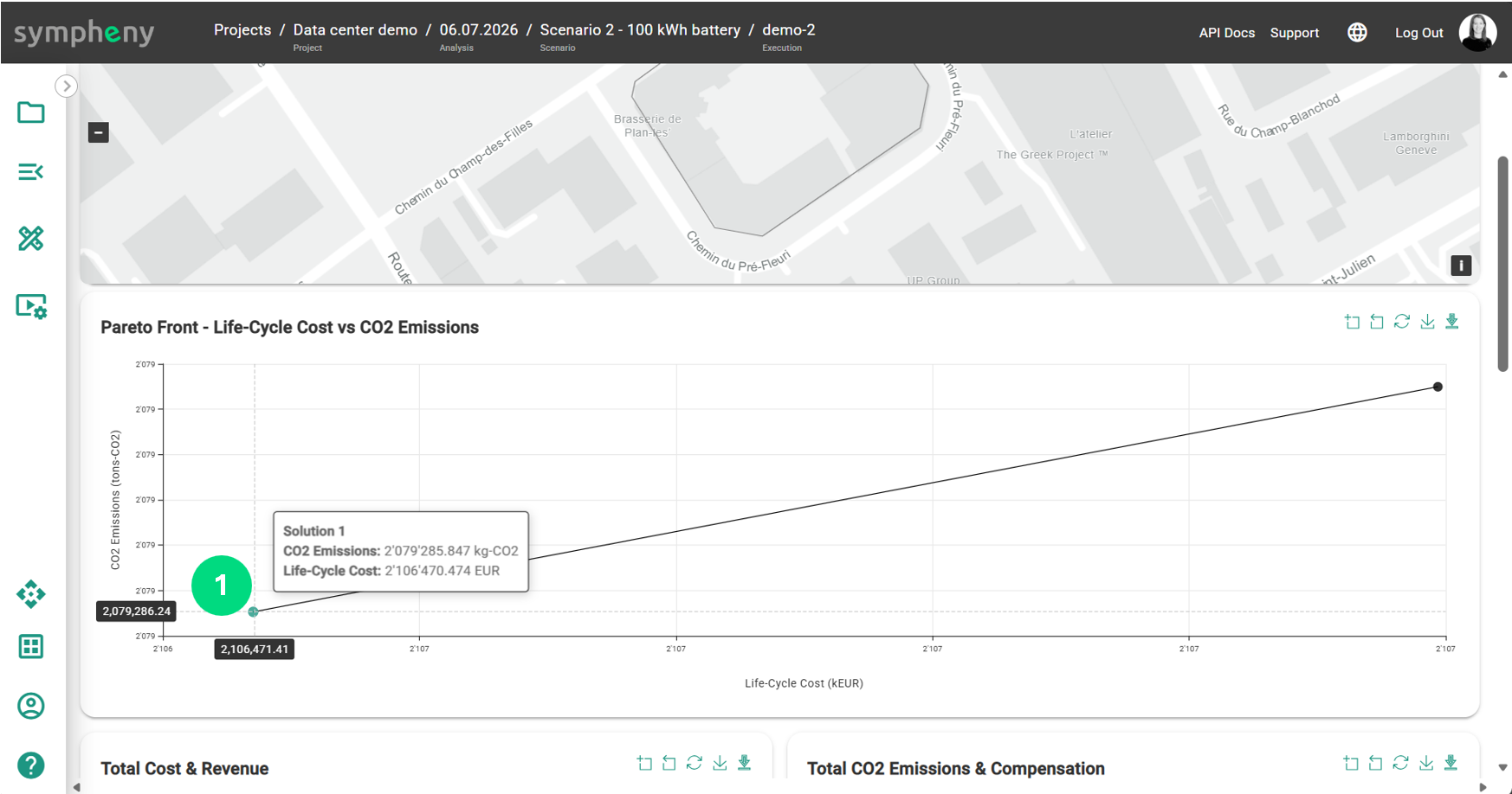
The Pareto Frond shows solution 1 and 2. We can see the total costs and missions of solution 1.
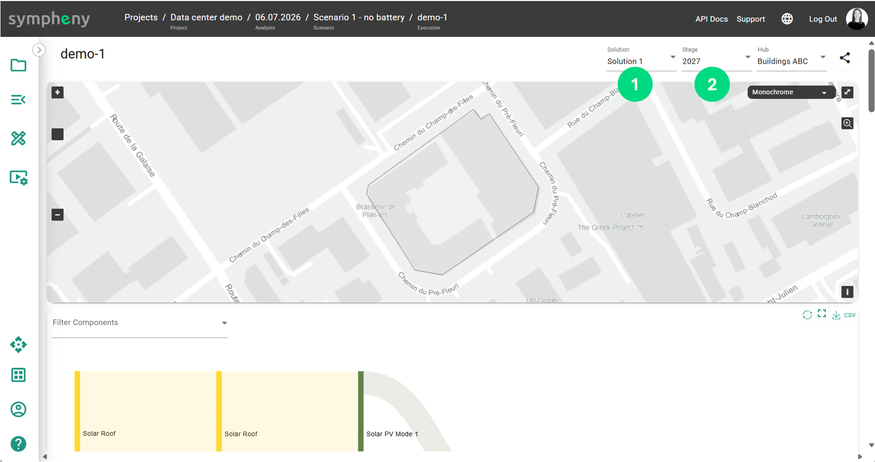
When we select Solution 1, the stage and the hub, we can view the detailed solution.
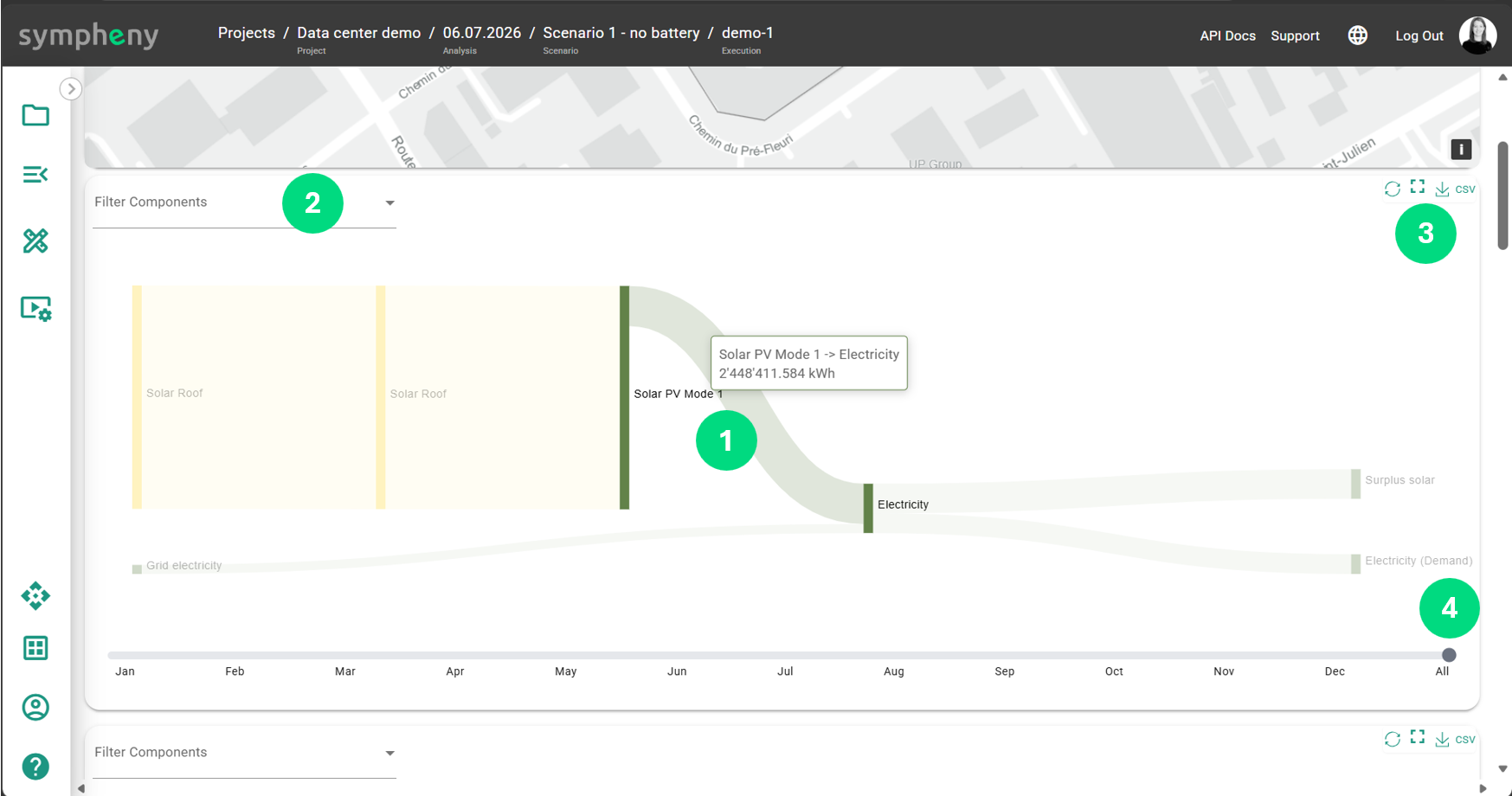
The Sankey diagram shows all of the energy flows in kWh. Like all diagrams, we can filter content, download data and images. The Sankey is also available for each month.
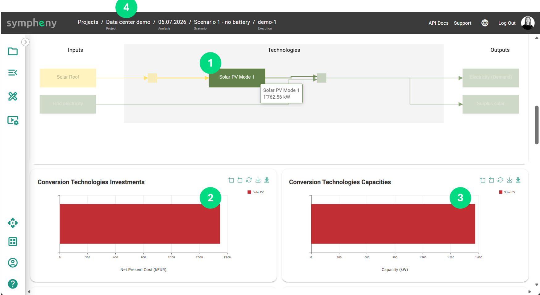
The energy diagram shows the capacity of each technology. In this cas the optimal size of the PV field is 1’760 kW (electric output). The investment of each technology is also available. We can use the navigation bar on top to go back to the scenarios.
We copy the scenario that we just created, to add a scenario with a battery.
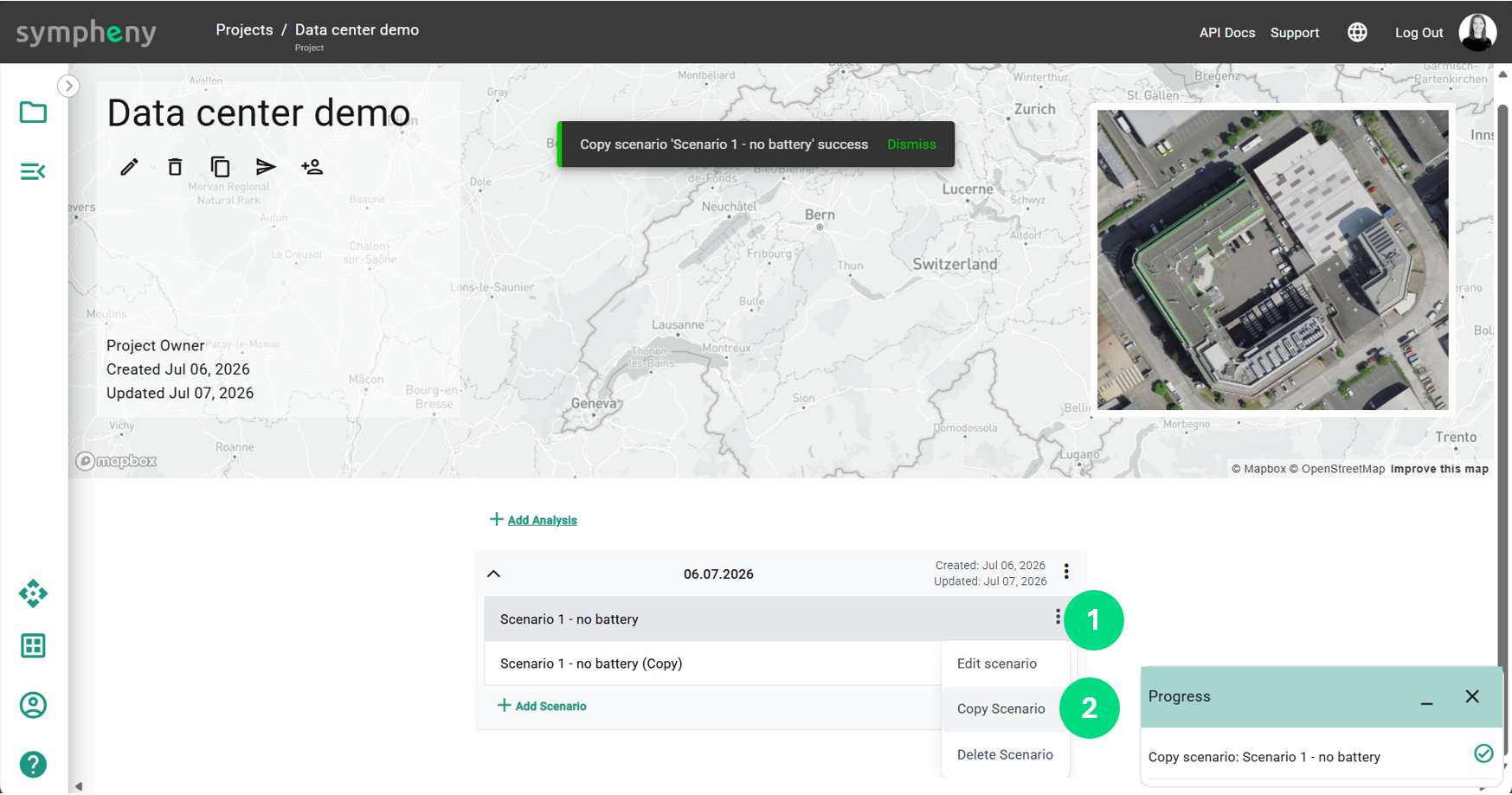
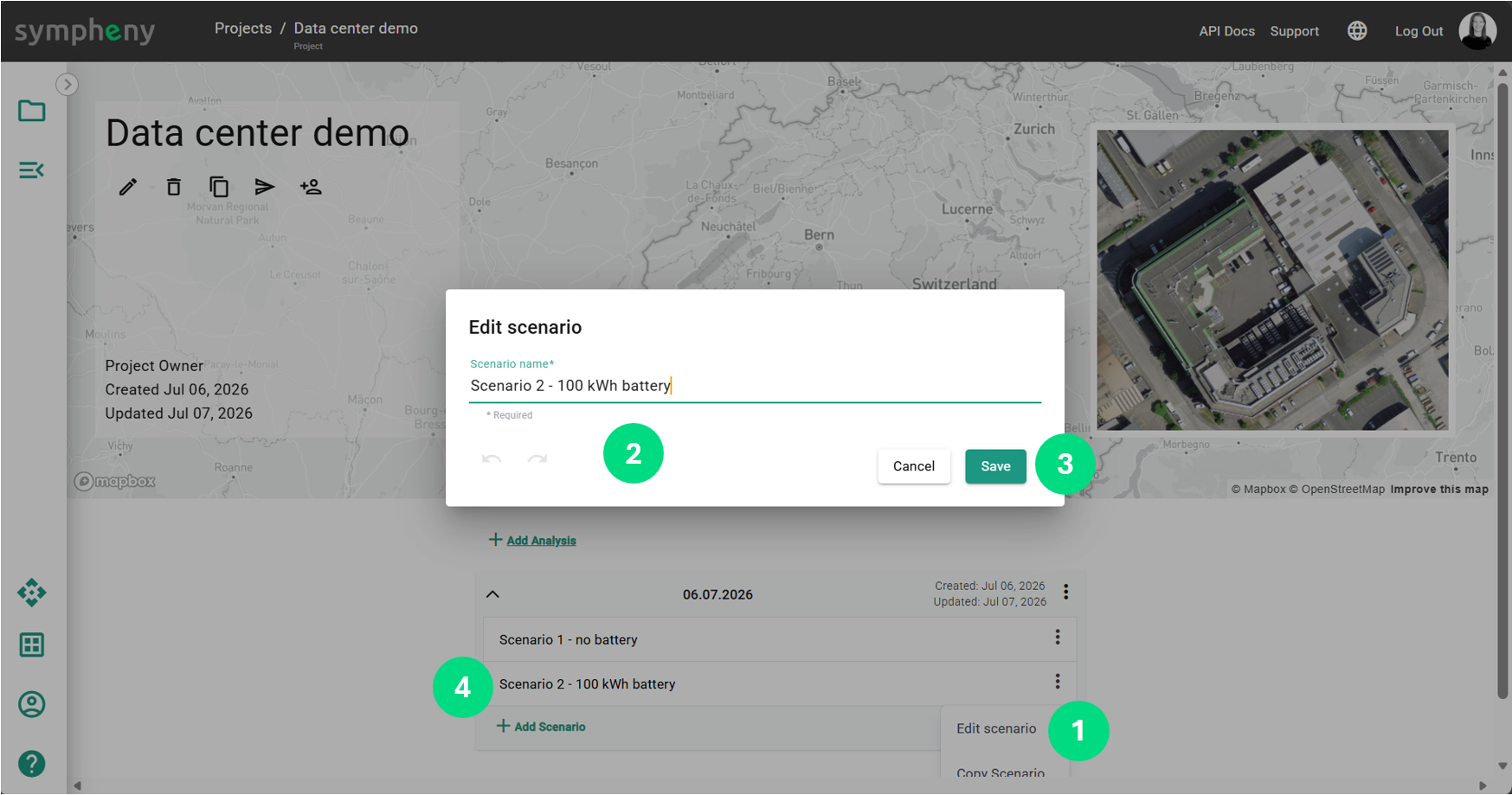
In this new scenario, all of the parameters have been maintained. So, we just need to add a battery.
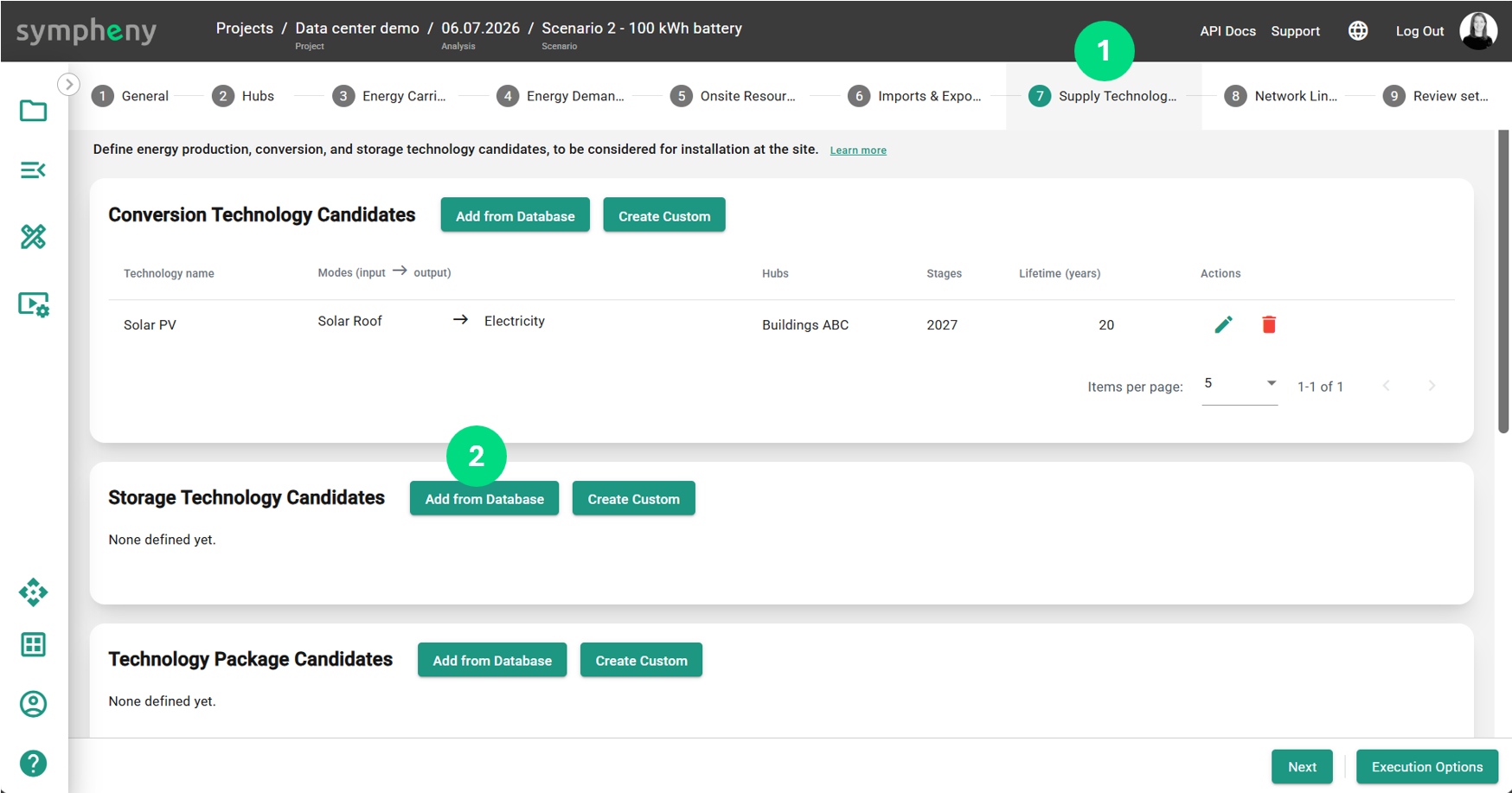
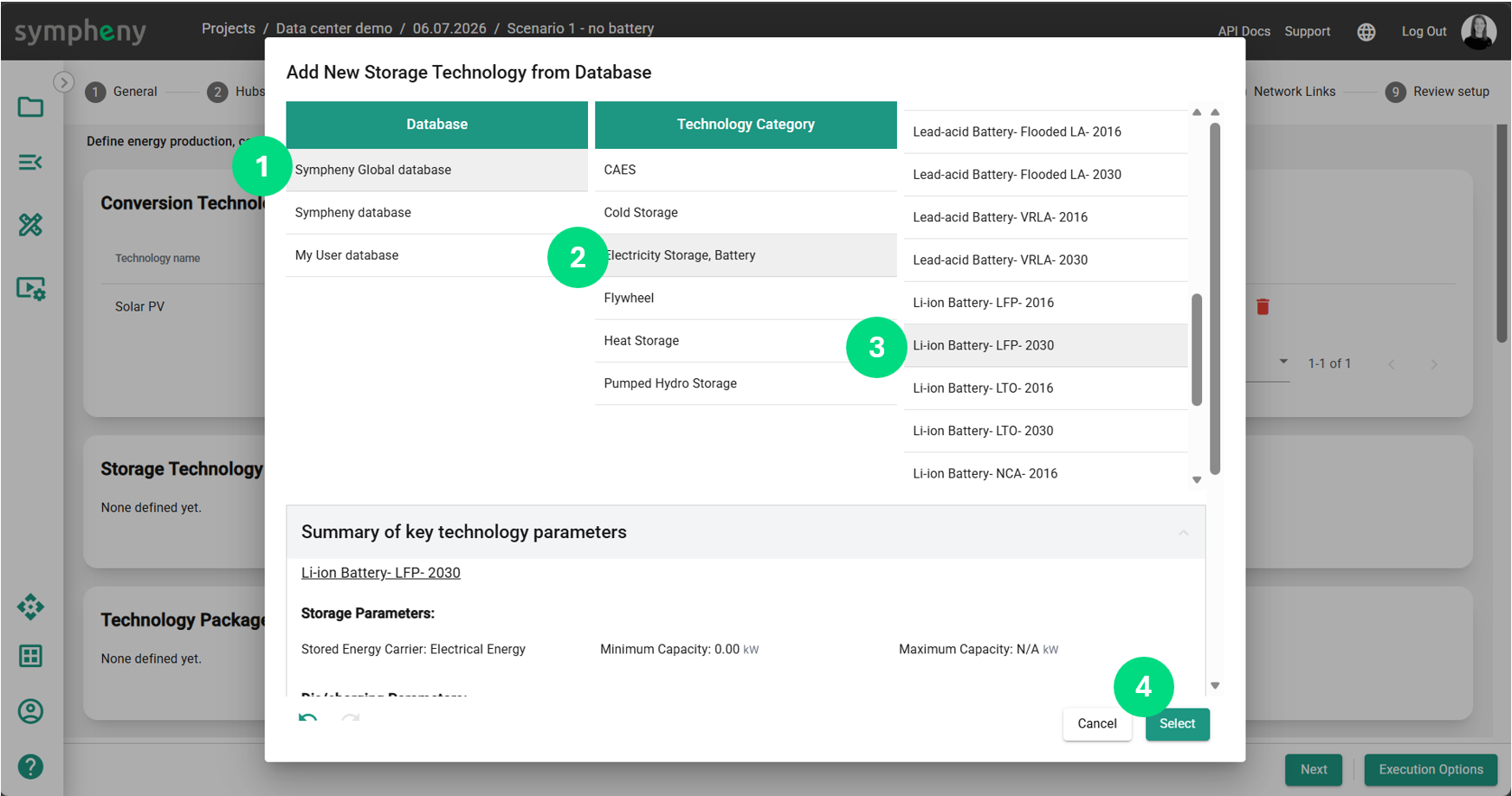
This time, we set it as must install and specify the capacity to be 100kWh. This constraint will be respected by Sympheny. The operation of the battery and the size of the solar field will be optimized.
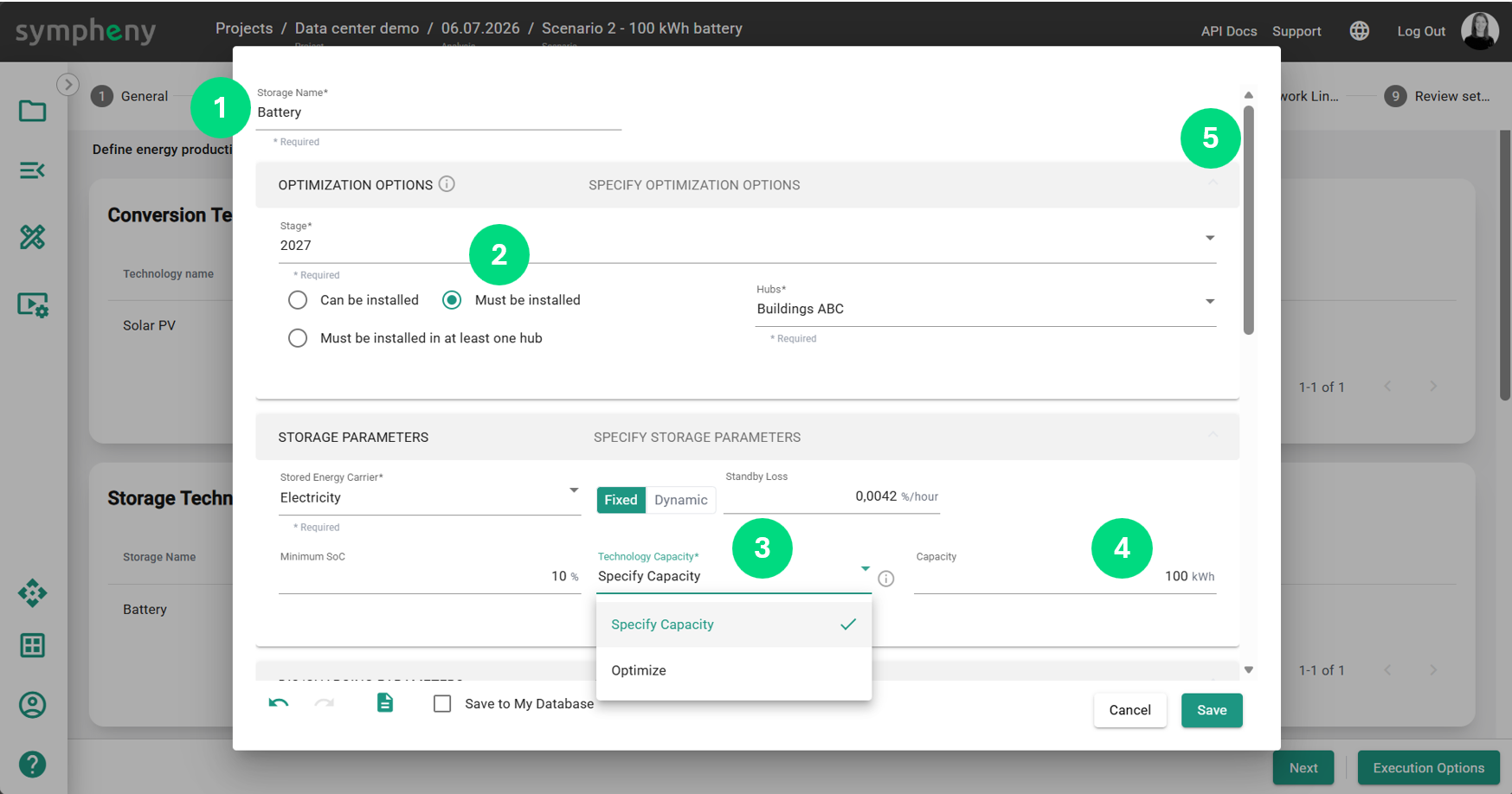
A different set of parameters are available for storage technologies.
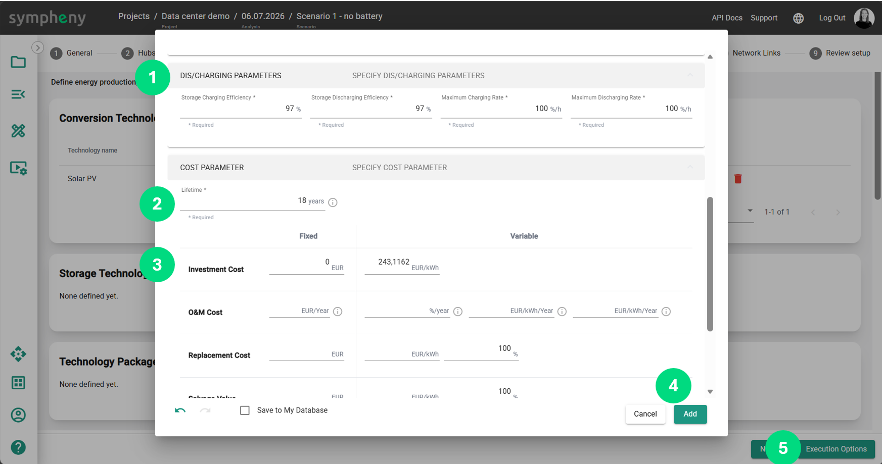
Once the battery is added, we execute the scenario with the same objectives and view the results.
If we select “All Stages”, we see that the result for cost and emissions is slightly better with the battery.
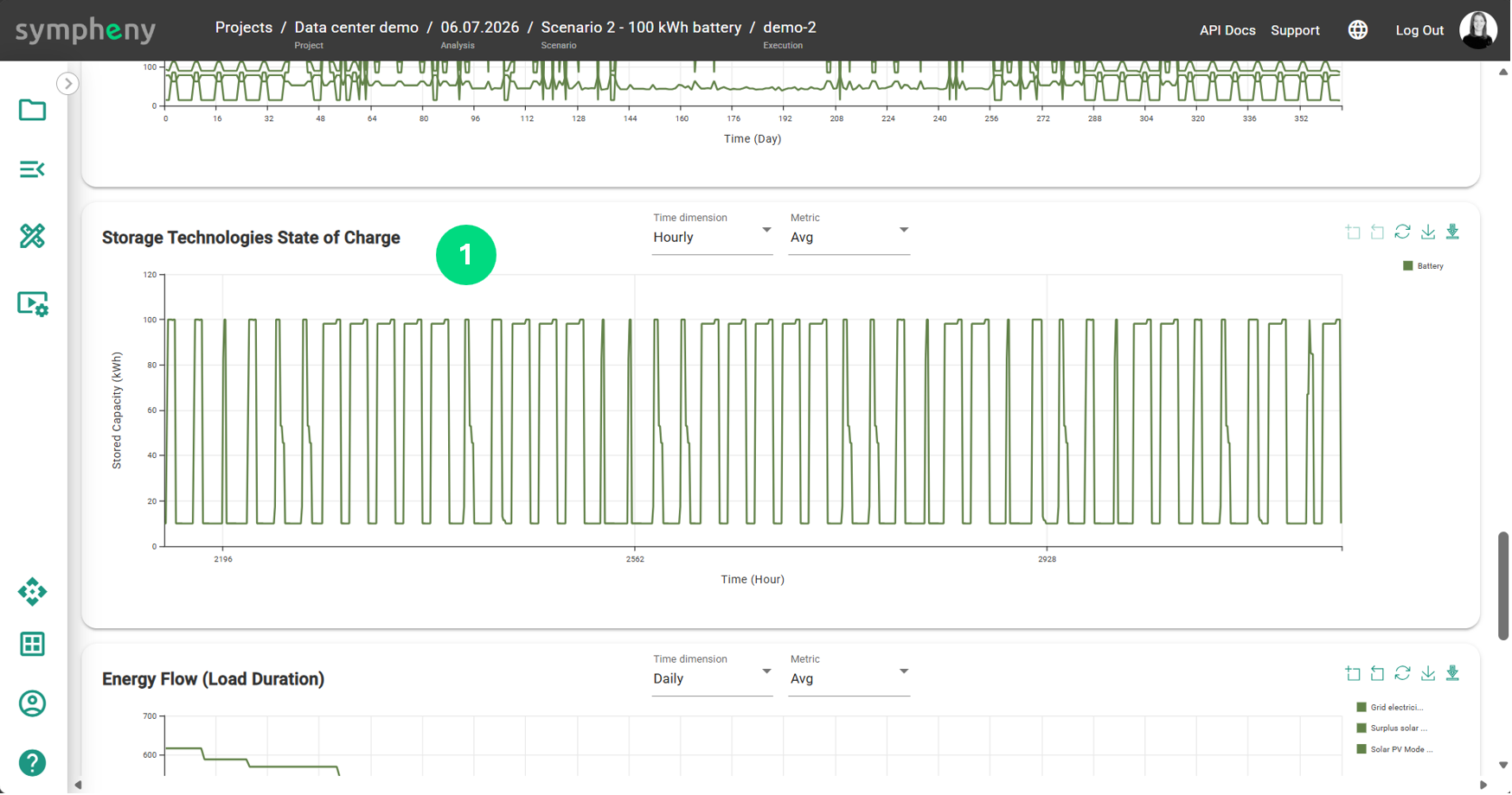
In the detailed results, we can see the hourly state of charge of the battery, in this view, we zoomed in on a specific month.