Tutorial 1 - Example case (Set-up)

Overview

This tutorial will show you how to implement the following features in your energy model:

> Basic conversion technologies: PV panels and Gas Boiler

> Multi-input technology: Air-source Heat Pump

> Multi-output technology: Gas CHP

> Storages: Battery and Hot Water Tank

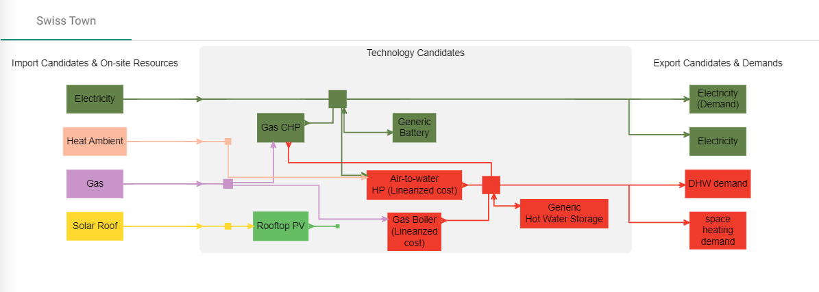
The energy hub system diagram below illustrates the energy system we will model in this tutorial:

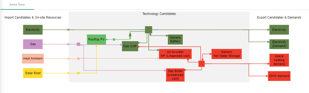
The blocks on the right side of the diagram, under Export Candidates & Demands, reflect energy demands which have to be satisfied (e.g. the blocks with Demand in their names) as well as potential energy exports out of the system boundary (e.g. the block Electricity).

The blocks on the left of the diagram, under Import Candidates & On-site Resources, reflect the resources which can be imported and/or utilized on-site (e.g. Solar Roof and Heat Ambient).

Finally, in order to be able to supply the requested energy demands to the site, Technology Candidates must be created. They can be conversion technologies (e.g. Rooftop PV) or storage technologies (e.g. Battery). The system diagram is generated automatically as each technology is created in the Sympheny web-app, this diagram provides an easy overview on how the different energy streams are linked and transformed.

The system diagram only appears once you will have added your first technology, i.e. once you reach the step 7 - add supply technologies.

For more information, do not forget to have a look at the fully searchable https://support.app.sympheny.com/user-guide/latest/. If you have any further questions, do not hesitate to e-mail us at support@sympheny.com.

Step 0 – Creating a new scenario

> Login to the webpage https://app.sympheny.com/login to start constructing your model.

> Click on the circled plus symbol (⊕) and name your project  Example Case to create your own project on your Projects page. Click Save.

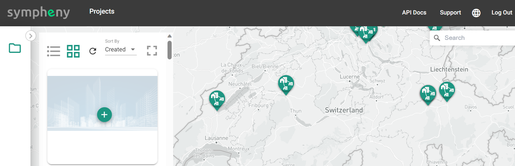
> Select your project by clicking open to go to the Analyses page. Add an analysis by pressing ⊕ and name it Energy Strategy 2050. Press Enter.

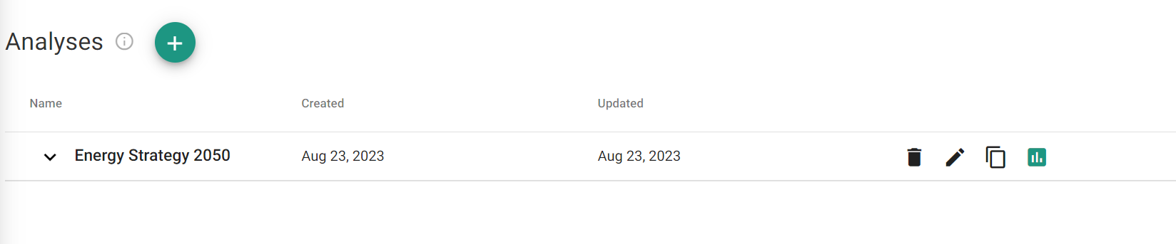
> Select the analysis Energy Strategy 2050 and add a scenario by pressing ⊕ and name it Baseline. Press Enter.

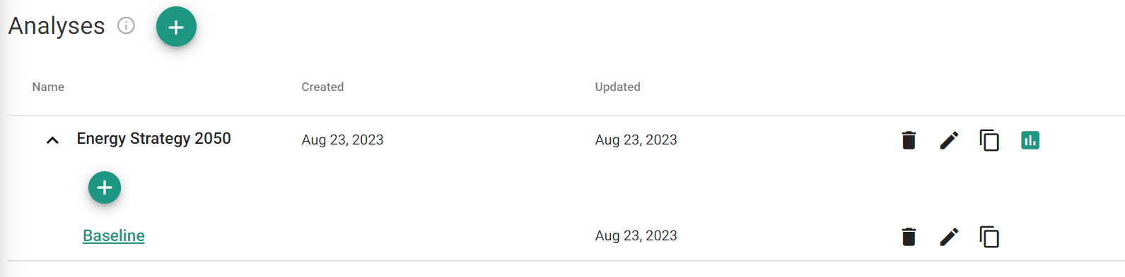
> Select the scenario Baseline to open the set-up page. Let’s start setting up your model!

Step 1 - General

In this tutorial, the interest rate is left to 0% and the currency to CHF.

Step 2 - Hubs

The hub section allows you to create different energy hubs. A hub is an energy-node: it can produce and or consume energy and different energy conversion and storage technologies may be installed in each hub. What it represents is up to you: a hub can represent a single building or a group of buildings depending on the scale of your analysis.

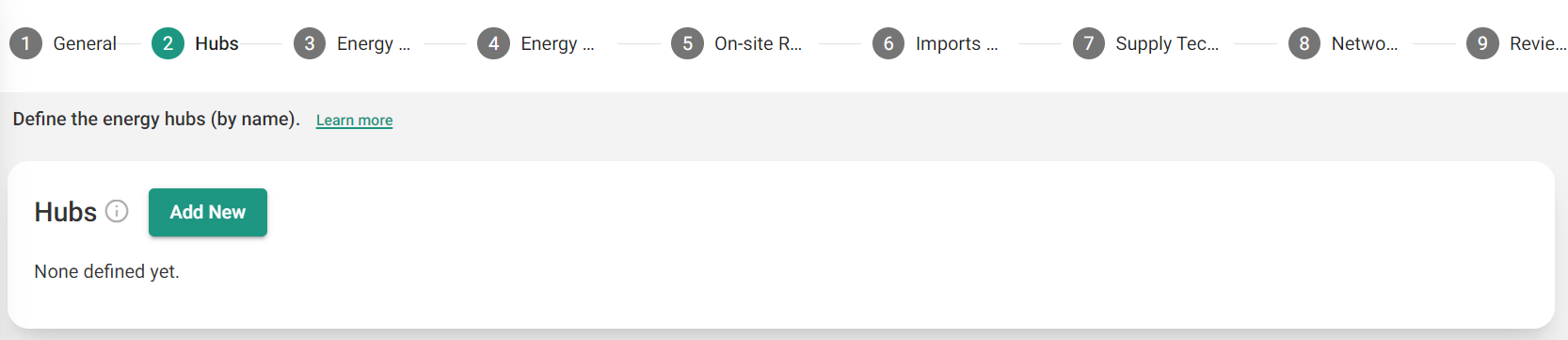
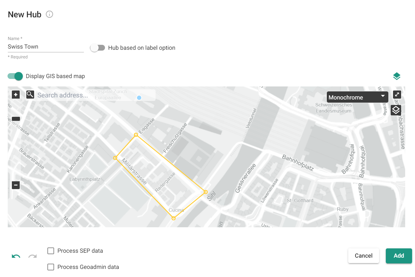
> Select Add New, name it Swiss Town and press Add.

Optional: By activating the toggle 'Display GIS based map', the hub can be drawn on the map. In the search address bar, enter your address and then draw the hub on the map (reminder: it can be a single buildings or a group of buildings).

> Press Next on the lower right corner to move to the Energy Carriers (EC) section. You can also simply click on the second step at the top.

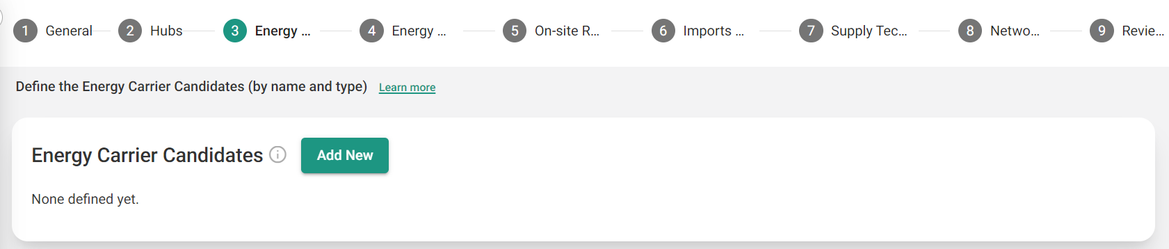
Step 3 - Energy Carriers (EC)

The energy carrier section allows you to define all the energy carriers that you will later use in your system. Think of this as a library of all the energy carriers you might be using later on and note that you can always come back to this step to add some more.

> Select Add New to define an energy carrier.

> The table below displays energy carriers used in this tutorial. Assign the Type, Subtype and Name of each energy carrier and select Add. Repeat the procedure for each energy carrier.

> Now you have added all the ECs, please click Next to move to the Energy Demands section.

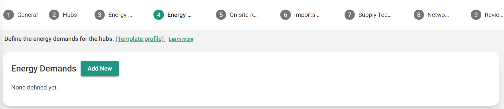
Step 4 – Energy Demands

Under the step Energy Demands the energy demand of your site are entered as hourly profiles for one year.

> Press Add New to add an energy demand.

> Select the Hub where the demand profile is located and the corresponding Energy Carrier. 

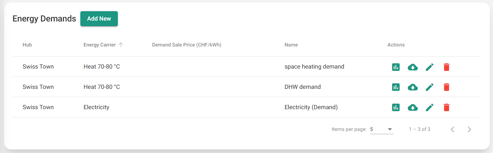
Optionally, a Name for the demand profile (e.g. space heating demand) can be specified as well as a Demand Sale Price. The Demand Sale Price generates an income to the system when the corresponding demand is supplied and is specified in CHF/kWh. In this example, we assume that the system is paid for by the same entity that will consume the energy on-site, hence the Demand Sale Price is left blank (meaning to the revenue is generated through the sale of the energy produced on-site).

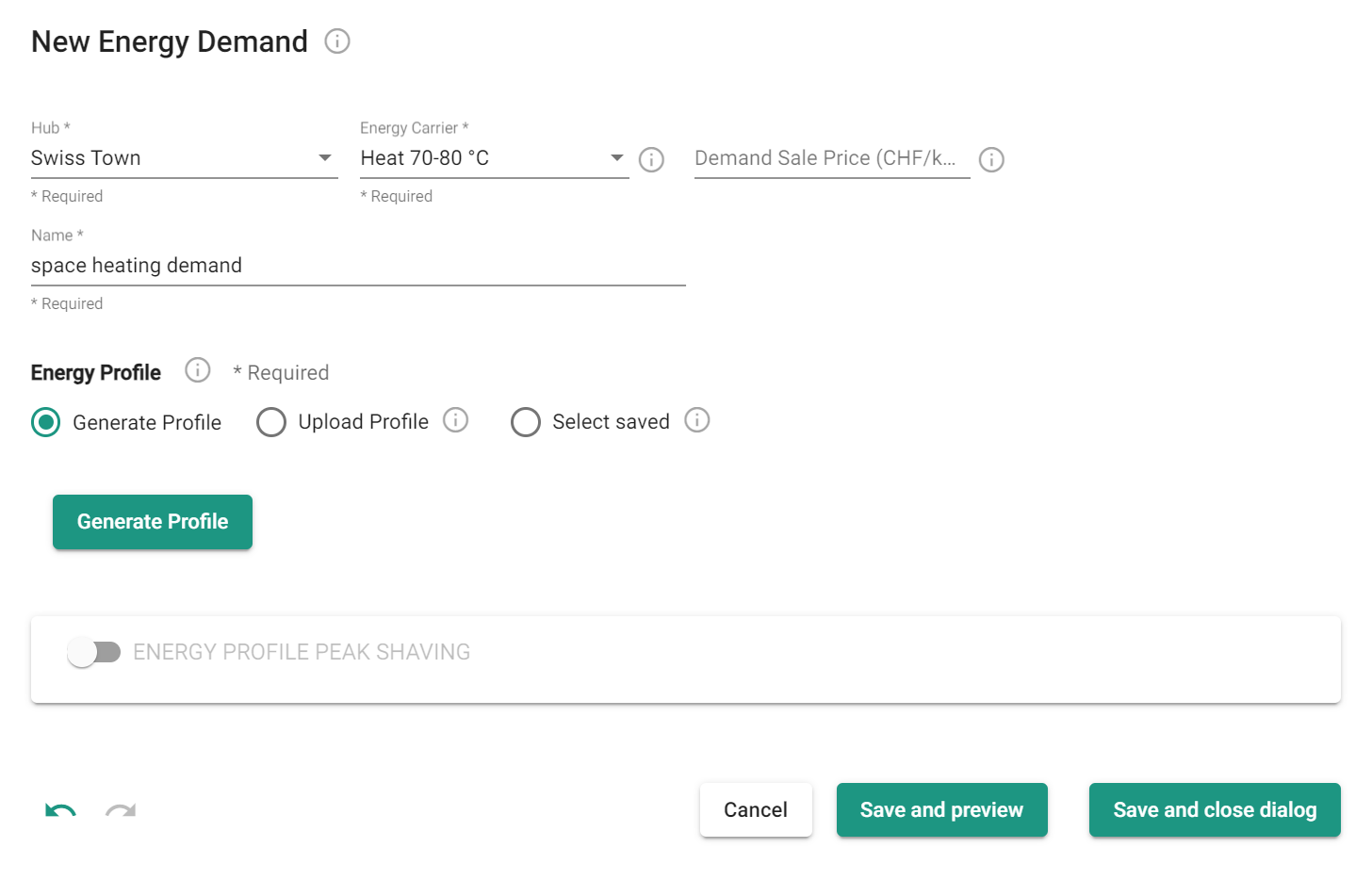
The energy demand profiles for a site may be specified in 3 ways (please refer to the https://support.app.sympheny.com/user-guide/latest/ section Add Energy Demands for more information):

• Generate Profile: select a profile from our in-house database (will be used in this example)

• Upload New: upload your own excel profile

• Select saved: select a profile from your personal database

> Press Generate Profile to generate your site-specific demand based on profiles saved within the database. Here, we want to model the demand profiles for 100 multi-family housings with the assumption of 100 [m2] per housing. For the Energy Carriers given below, select the following Demand Type – Building Use – Building Age combinations from the database:

• For the Energy Carrier Heat 70°C-80°C, select Space Heating – Multi-family House

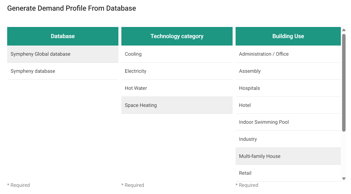
• Scroll down, select By Building Age and <1970 as the Demand Type. Finally, give it an Energy Reference Area of 10’000 [m2]

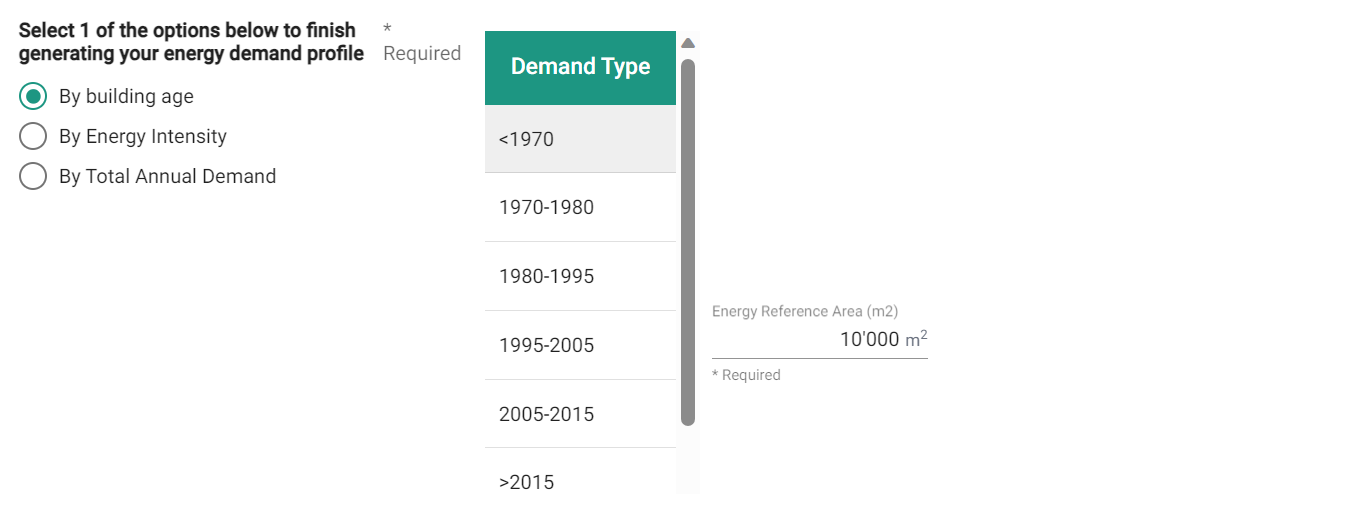
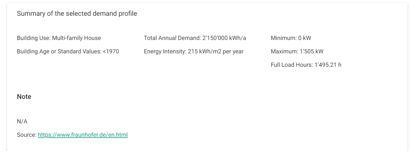
Note: if you scroll down until the bottom you the window, you will find summary information about the selected profile:

Repeat the steps for the two following entries (Hot water and electricity demand)

• Energy carrier: Heat 70°C-80°C: Hot Water – Multi-family House – By Building Age - <1970

> Give it an Energy Reference Area of 10’000 [m2] and select Next. Then press Add. Follow the same steps with Electricity as your Energy Carrier (Add New – select Hub – Energy Carrier – Generate Profile)

• Energy carrier: Electricity:  Electricity – Multi-family House – By Building Age - <1970

> Give it an Energy Reference Area of 10’000 [m2] and select Next. Then press Add.

You will hence end up with three energy demand entries:

Step 5 – On-site resources

All resources with intermittent availability (temporal variability), such as solar irradiation, are dealt with in this dedicated step.

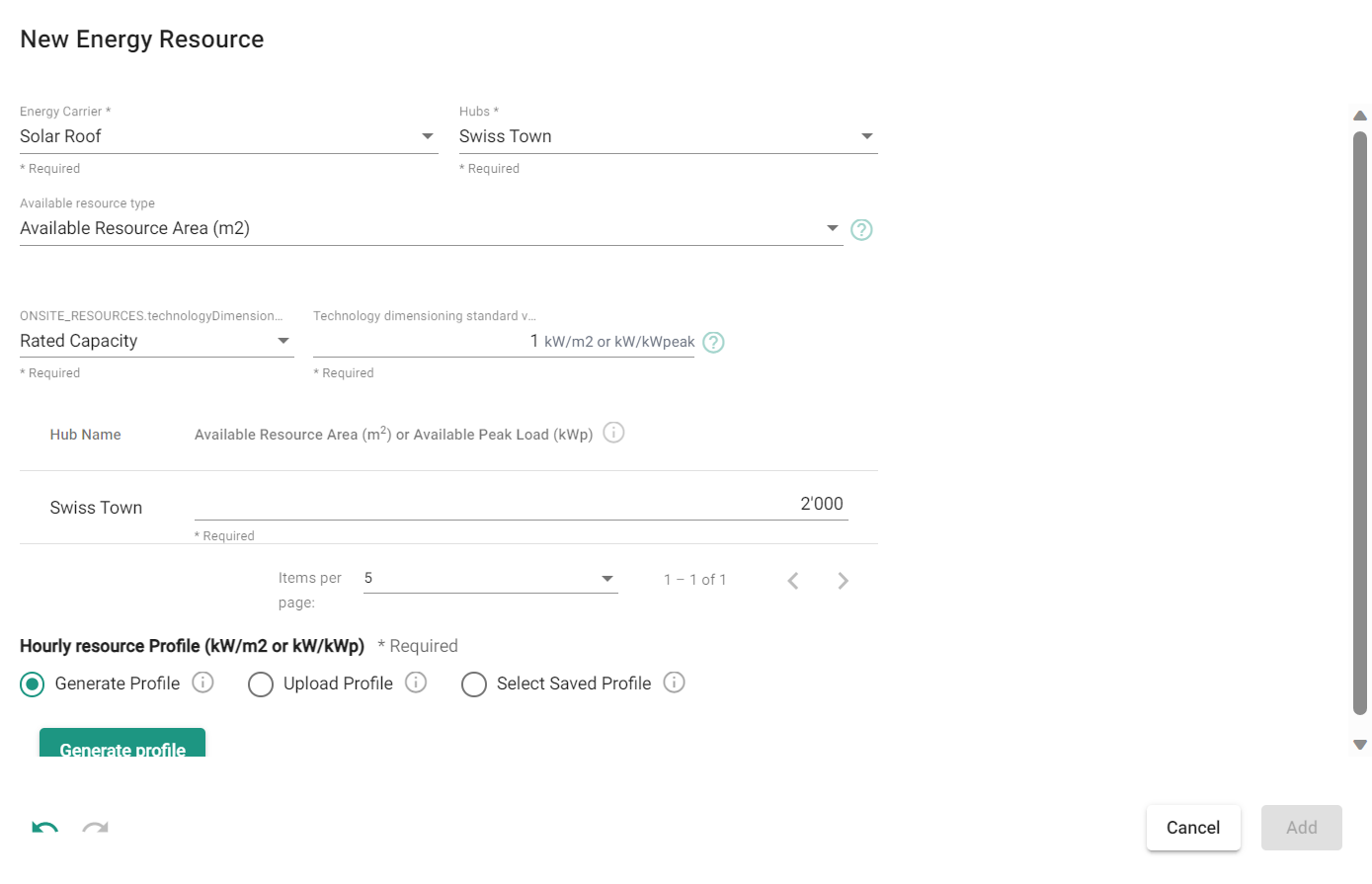
> Select Add New to add the solar irradiance available at your location

> Select the energy carrier Solar Roof and the Hub created before. Select Available Resource Area (m2) as your available resource type.

> Select Rated capacity and leave the Technology dimensioning standard value to 1 kW/m2.

This means that the dimensioning of the subsequent technology (= the technology having this resource as input) will be calculated based on the Technology dimensioning standard value, and not based on the profile maximal value. The variable costs of the technology will then also be based on this dimensioning.

This is standard for solar technologies, for which the capacity is calculated under Standard Testing Conditions (with an irradiation of 1 kW/m2). The calculation is the following:

Optimal_Capacity = Optimal_Sizing[m²] * Tech_Dim_Standard_Value[kW/m²] * Efficiency

For more information, please see the section Calculation example for solar irradiation as on-site resource (kW/m²) under https://support.app.sympheny.com/user-guide/latest/on-site-resource-candidates .

> Give an Available Resource Area of 2’000 [m2]

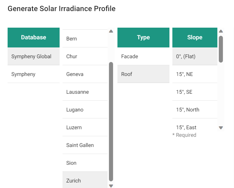
> Now select the availability profile to apply to your potential: press Generate Profile and select the following Location – Type – Slope & Orientation combination:  Zurich – Roof – 0°, (Flat), which corresponds to the irradiance profile for a roof with a slope of 0° (= flat). Press Next.

> Select Next to move to the Imports & Exports section.

How do I know if I should enter a profile in kW/m2 or in kW/kWp?
This depends on the unit of your data: they most important being that the units stay consistent.

• When entering a profile in kW/m2 (e.g. an irradiation profile at a certain location), the unit of the available resource is considered to be (m2), since the profile and the available resource unit will be multiplied together.

• On the other hand, if you enter a profile in kW/kWp, this underlies that your available resource is enter as an available peak load (kWp).

Step 6 – Import & Exports Candidates

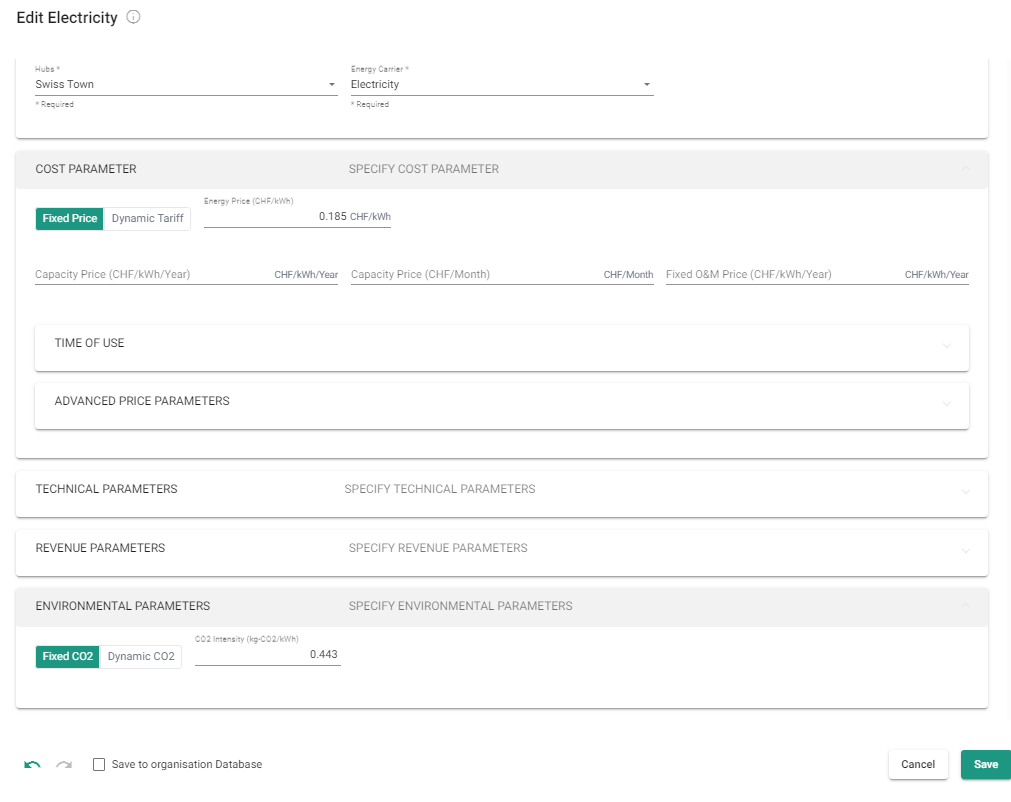
It is time to include imports and exports to your system. Each import may be assigned a price and a CO2 factor, each export a revenue and a CO2 compensation.

> Under Import Candidates select Add New

> Fill in the boxes for the Energy Carrier Electricity of the Hub Swiss town as follows and press Add:

• Energy Price [CHF/kWh] = 0.185

• CO2 Intensity [kg-CO2/kWh] = 0.105

> Repeat this step for the Energy Carrier Gas

• Energy Price = 0.08 [CHF/kWh]

• CO2 Intensity= 0.22 [kg-CO2/kWh]

> Finally, the Energy Carrier Heat Ambient also has to be ‘imported’ on-site. For this, simply create an import of the EC Heat Ambient, without cost nor CO2 factor.

> Under Export Candidates select Add New for the Energy Carrier Electricity. This means that you allow your system to export electricity, and are considering revenues for each kWh fed back to the grid:

• Energy Price (as revenue) [CHF/kWh] = 0.07

• CO2 Compensation : leave blank (or 0 [kg-CO2/kWh]), as now compensation is considered in this example

> Select Next to move to the Supply Technologies section.

Step 7 – Supply Technologies

Supply Technologies are divided between Conversion Technology Candidates or Storage Technology Candidates. ‘Candidates’ means that they are technologies that we want to consider for our site, but they will only be selected as part of the optimal system design solutions if the use of the technologies minimize the objective functions. In our case, the objective functions are life-cycle costs and life-cycle emissions.

They are two ways to create a technology model, either by using the Add from Database option, which will allow you to select technologies from a library with pre-defined parameters, or by creating a technology from scratch, using the button Create custom. We will go through both methods in this tutorial.

A technology package is a predefined combination of energy conversion and/or storage technologies which are commonly used or evaluated together. The technology packages will not be used in this tutorial.

7.1 Modelling conversion technologies

Step 7.1.1 Modelling PV Panels

> Select Create Custom under the conversion technology candidates area and fill the parameters with the following data:

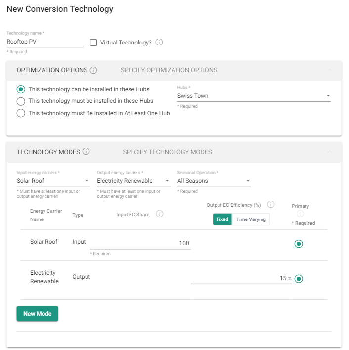
> Press Add.

The input EC of the Rooftop PV technology is on-site resource ‘Solar roof’. As we selected ‘Rated capacity’, the costs for the PV will be based on the following optimal capacity:

Optimal_Capacity = Optimal_Sizing[m²] * Tech_Dim_Standard_Value[kW/m²] * Efficiency

in this case, this means:

Optimal capacity (from results) = Optimal sizing in m2 * 1 * 0.15

It is as such possible to recalculate the surface area required:

Optimal sizing in m2 = Optimal capacity (from the results) / 0.15

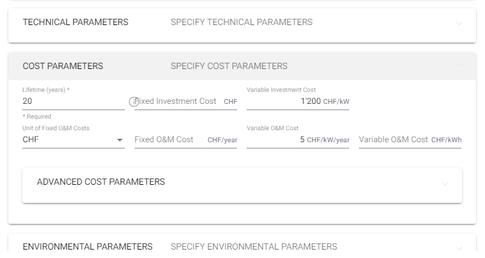
You can also select a minimum capacity of PV to install under the Technical Parameters section, Minimum Capacity (kW). This refers again to the optimal rated capacity.

If you’d like to save the technology to your personal Database, check the box ‘Save to My Database’ and enter the information required after pressing Add.

As you might have noticed, costs of technologies represented as a linear ‘cost curves’. For example, the investment required for a technology is given as such:

Fixed Investment costs [CHF] + c * Variable Investment costs [CHF/kW], with c representing the optimal capacity, as calculated by the optimization algorithms.

For more details as to the creation of such a cost curve, please refer to our video (in German):

https://www.youtube.com/watch?v=dakbFBlUFQg

Step 7.1.2 Modelling a Gas Boiler

> Select Add from Database and select the following:

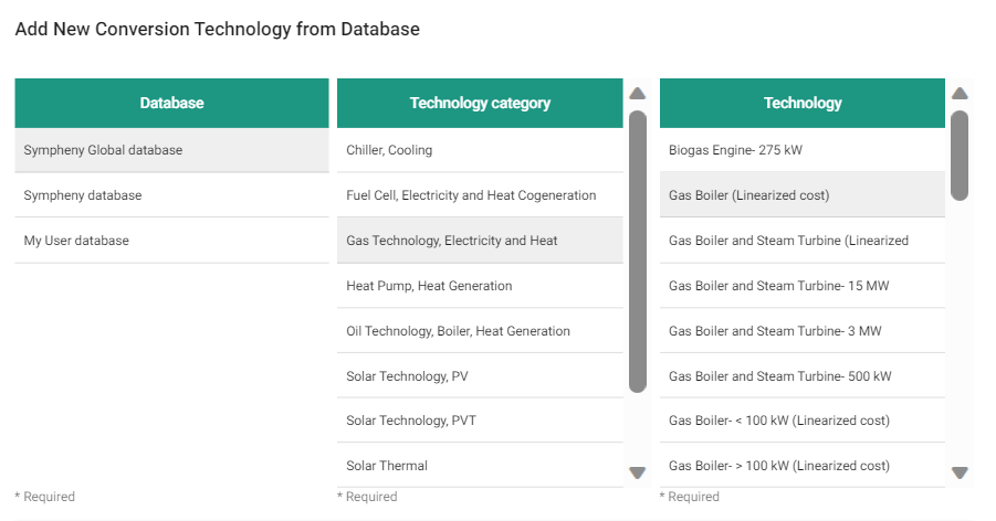
> Press Select

> Select the corresponding hub in which the technology may be located (in this case, the one and only hub, Swiss Town).

> Take a look at the values entered, modify them if you’d like, and press Add.

Step 7.1.3 Modelling a simple heat pump (multi-input technology)

> Select Add from Database and select the following:

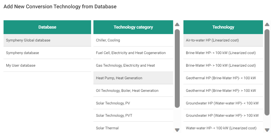
> Press Select

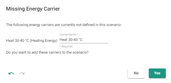
> A Missing Energy Carrier Panel will appear (see below). This is due to the fact that the technology Air source heat pump has been saved in the database with the Energy Carrier ‘Heat 30-40°C’. This can be changed after. Hence, press yes first.

> Select the corresponding hub.

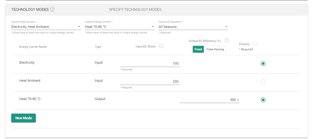
> Under the section Technology Modes, note that two Energy Carriers are selected as Input Energy Carriers: Electricity and Heat Ambient.

> Still under the section Technology Modes, click on the drop-down menu of the field Output Energy Carrier:

first, unchecked the EC Heat 30-40°C

second, check the EC Heat 70-80°C

While doing so, the Output EC efficiency (%) will automatically be set back to 100%. Make sure that you change it back the value of 300% (as defined in the database).

> Press Add.

The 300% efficiency given here, corresponds to a yearly COP of 3.

The calculation is done as such:

Units Primary Input (=Electricity) + Units Secondary Input (=Heat Ambient) = Output EC efficiency (=Heat 70-80°C) * Units Primary Input

leading in our case to 100 units Electricity + 200 units Heat Ambient producing 300% * 100 = 300 units Heat 70-80°C, hence a COP of 300/100 = 3. 

Step 7.1.3 Modelling a Gas CHP (multi-output technology)

This step consists of modelling a Gas CHP (Combined Heat and Power), which generates two outputs: Heat 70-80°C and Electricity, i.e. both outputs will have to be selected as Output Energy Carriers under the Technology Modes.

> Select Create Custom once more and fill in the boxes like given below:

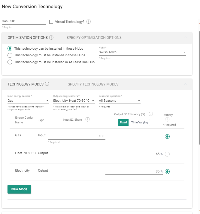
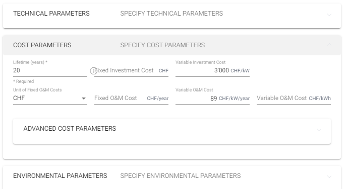
Since the CHP has two outputs, one of them must be defined as the primary output. The primary output is the output which will be relevant for the capacity and consequent cost calculation of the technology, in this case, Electricity. Note that it does not mean that the technology operation is controlled by the electricity demand, the operation is always based on what leads to the optimal objective functions (in our case, costs and emissions).

Step 7.1.4 Modelling a Transformer as a virtual technology

At this stage, your system diagram should look like this:

As you might notice, the output of the technology Rooftop PV is not linked to another technology or sent to “Export Candidates & Demands”. This will cause an error as there is no way to close the energy balance in the calculation.

In the model of Rooftop PV, the output EC is Electricity Renewable (line colored in light green), while the system has a demand set as Electricity (line with a dark green color). If we want the rest of the system to utilize Electricity Renewable as Electricity, we need to create a technology to convert Electricity Renewable to Electricity. Here is how to do that:

> Select Create Custom once more and fill in the boxes like given below:

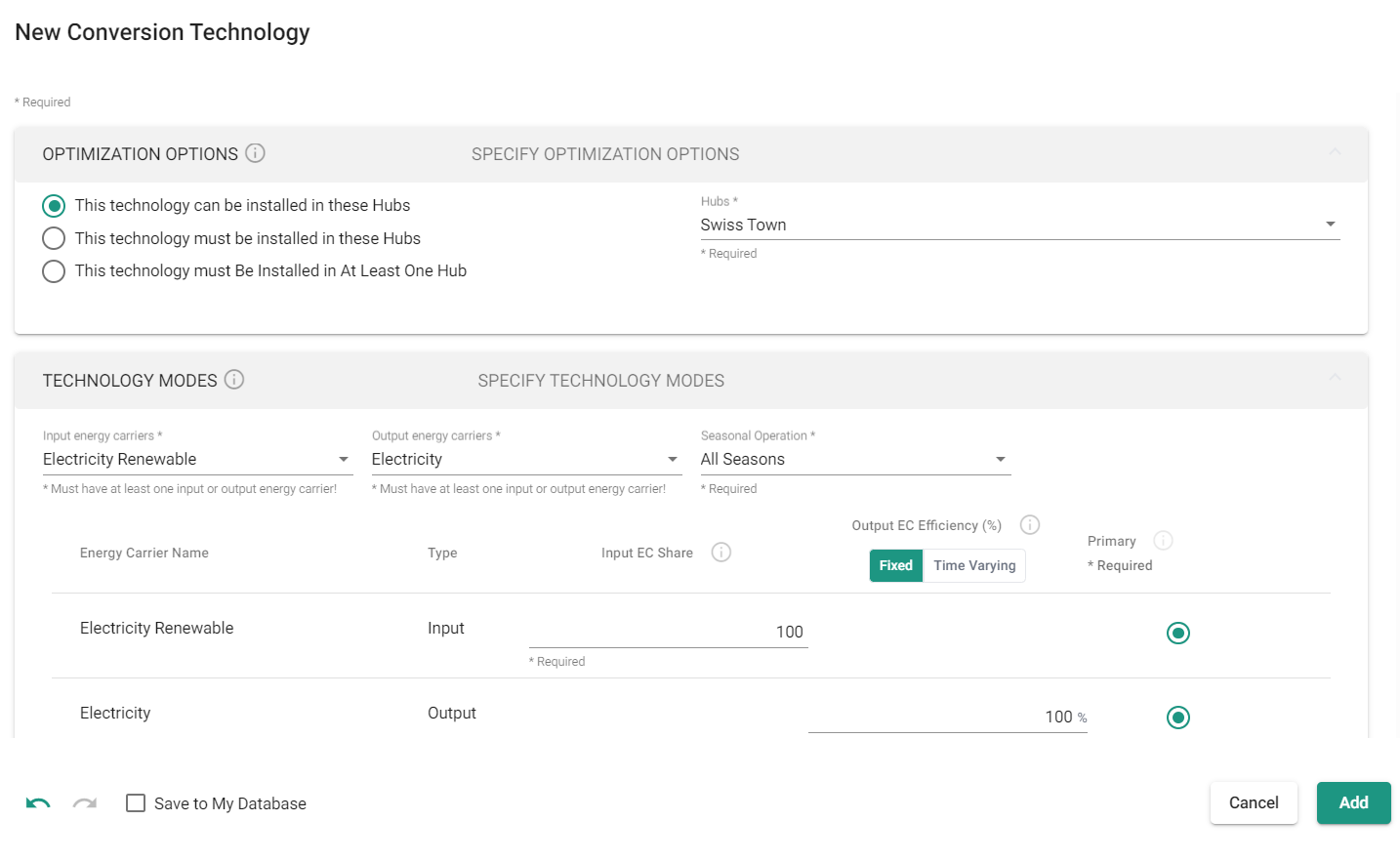
By checking the box ‘Virtual Technology’, you create a technology without costs. This technology can be seen as a ‘translator’: you allows the EC Electricity Renewable to be ‘translated’ to the EC Electricity, without incurring any cost in the total accounting.

> Select Add

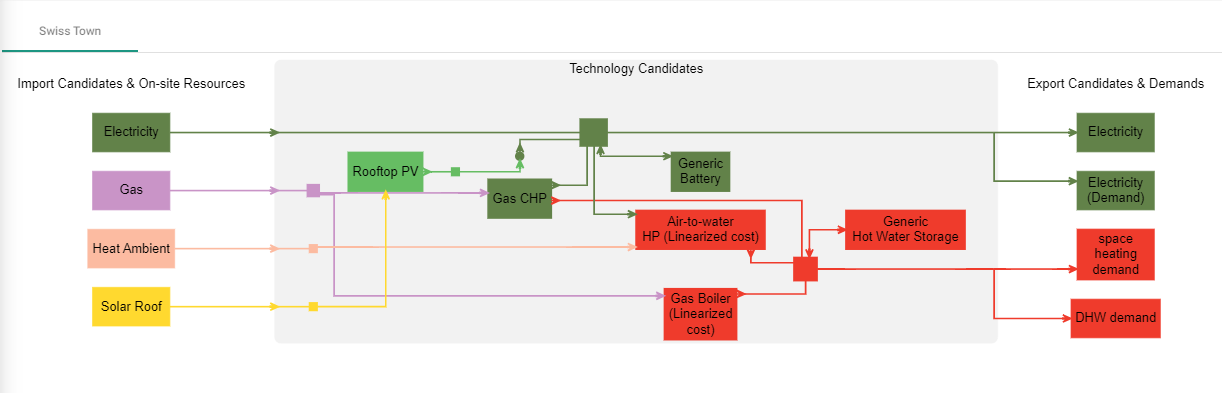
Notice now how the energy flows are connected in the system diagram. Virtual technologies (VT) are represented by a dot in the system diagram.

7.2 Modelling storage technologies

7.2.1 Modelling of a battery

> Select Add from Database and select the following:

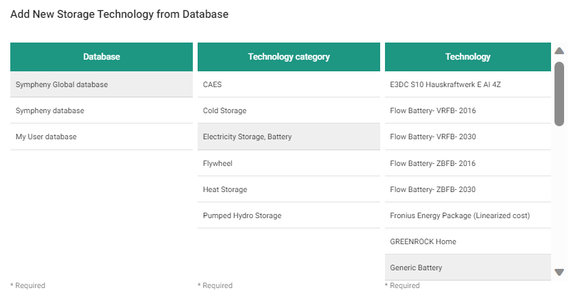
> Press Select

> Select the Hub

The battery’s Maximum Capacity in kWh should be limited to a certain extent. Indeed, if no maximum capacity is entered, it is likely (depending on the input parameters) that the optimal solution in terms of emissions models would be the use of the battery as a seasonal storage, which is not the desired output.

> Under Storage Parameters, set the maximum Capacity (kWh) to 500 kWh.

> Press Add

7.2.2 Modelling of a Heat Storage

Repeat the procedure to add the Heat Storage:

> Select Add from Database and select the following:

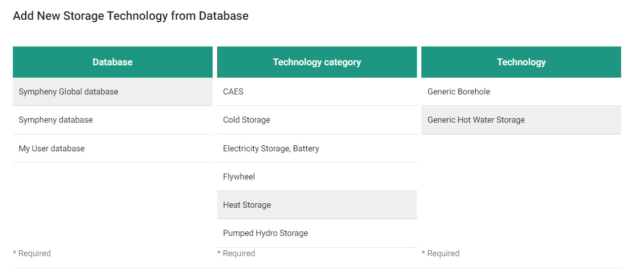
> Press Select

> Select the Hub

> Press Add

Step 8 – Network Technologies and Links

Network Technologies and Links are used to model the pipes used to share an Energy Carrier between different Hubs. This tutorial has only one Hub and won’t need any Links.

> Select Next to move to Other.

Step 9 – Review

Your set-up is now finished. This review section gives an overview over the entire scenario specification and allows editing of a section if necessary. If you scroll down, you can also compare your system diagram with the one below.

> Keep the Optimization Granularity to Medium. For more information to the Optimization granularity, please visit this section of the user guide: https://support.app.sympheny.com/user-guide/latest/review-your-model .

> Select Finish Specification & Prepare for Execution to get to the execution of the model.

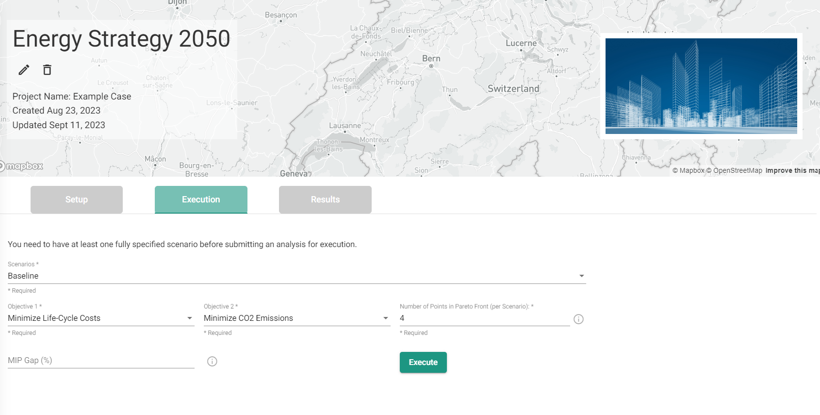
Step 10 – Execution & Results

Next to the Setup section you can find the Execution section where you select the Baseline scenario to be optimized and the amount of optimal solutions you would like to compare in detail ( = number of points in the pareto front), here 4. The more pareto points you have the more precise your pareto front (curve) will be, but the more solutions you have to compare and the longer the execution will take.

> Press Execute to start the optimization.

> Once you receive an email that the optimization is completed, click on the link which will bring you to the Results section. Alternatively, click on the Results tab and the Refresh button. Once the Status Message is set to DONE, you will be able to access your results, by clicking on View Results and then on View to open the dashboard. This section of the user guide will further help you with the understanding of the different visualizations: https://support.app.sympheny.com/user-guide/latest/results-dashboard .

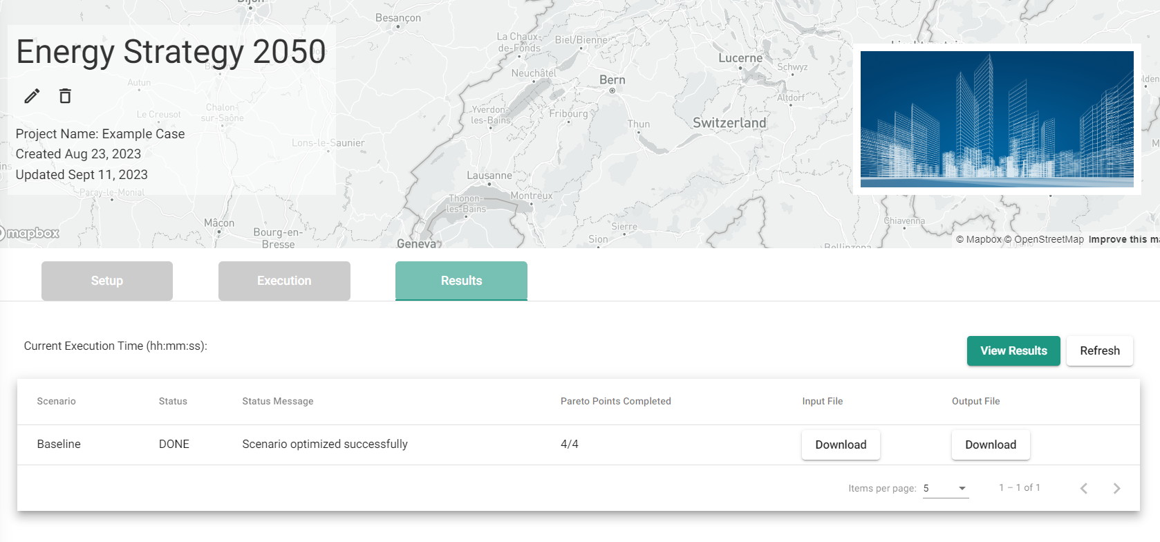
Tip: In the results section of your scenario, you can download the input.xlsx file. This file gathers all the boundary conditions of the specific scenario and allows an complete overview of your inputs.

You have further questions?

We hope that this tutorial was useful !

For more information, do not forget to have a look at the https://support.app.sympheny.com/user-guide/latest/. If you have any further questions, do not hesitate to e-mail us at support@sympheny.com.