
Free Cooling
- Free Cooling (with Geothermal Storage)
Based on the example of the Geothermal heat pump, let’s now consider that the cooling demand can also be supplied by free cooling, whenever this is possible. For doing so, a free cooling heat exchanger must be added. It is modelled as a separate technology, as we have already 3 modes in our brine-water heat pump technology (the current maximum number of modes).
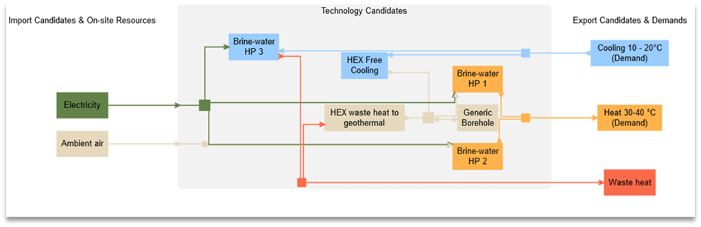
Figure 49 System diagram of Free Cooling with geothermal storage
Set-up summary
Energy Carriers | Energy Demands | Imports | Exports | Supply technology | ||||||
Brine water HP 1 | Brine water HP 2 | Brine water HP 3 | HEX waste heat to geothermal | HEX Free cooling | Generic Borehole | |||||
Electricity |
| X |
| Primary Input | (primary) Input | Primary Input |
|
|
| |
Geothermal heat |
|
|
| Input |
|
| (primary) output | Output | X | |
Ambient heat |
| X |
|
| Input |
|
|
|
| |
Heat 30-40°C | X |
|
| (primary) Output | (primary) Output |
|
|
|
| |
Cooling 10-20°C | X |
|
|
|
| (primary) output |
| (primary) output |
| |
Waste heat |
|
| X |
|
| Output | (primary) input |
|
| |
Set-up implementation
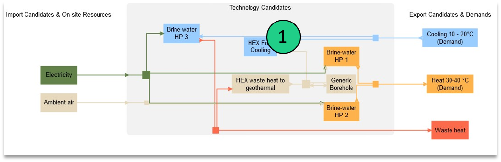
Figure 50 Set-up implementation of free cooling with geothermal storage
The free cooling has only two outputs, as it simultaneously creates cooling and heating by transferring heat from one medium to the other. The output of the free cooling HEX is directly the geothermal heat. This way, the technology can only operate when the geothermal sink is not fully loaded. For simplicity, pump electricity has been ignored. Of course, adding an electricity input and strongly increasing the efficiency of the outputs would allow to consider it (e.g. for an output efficiency of 1’000 %, 1 unit of electricity would be needed for producing 10 units of cooling).
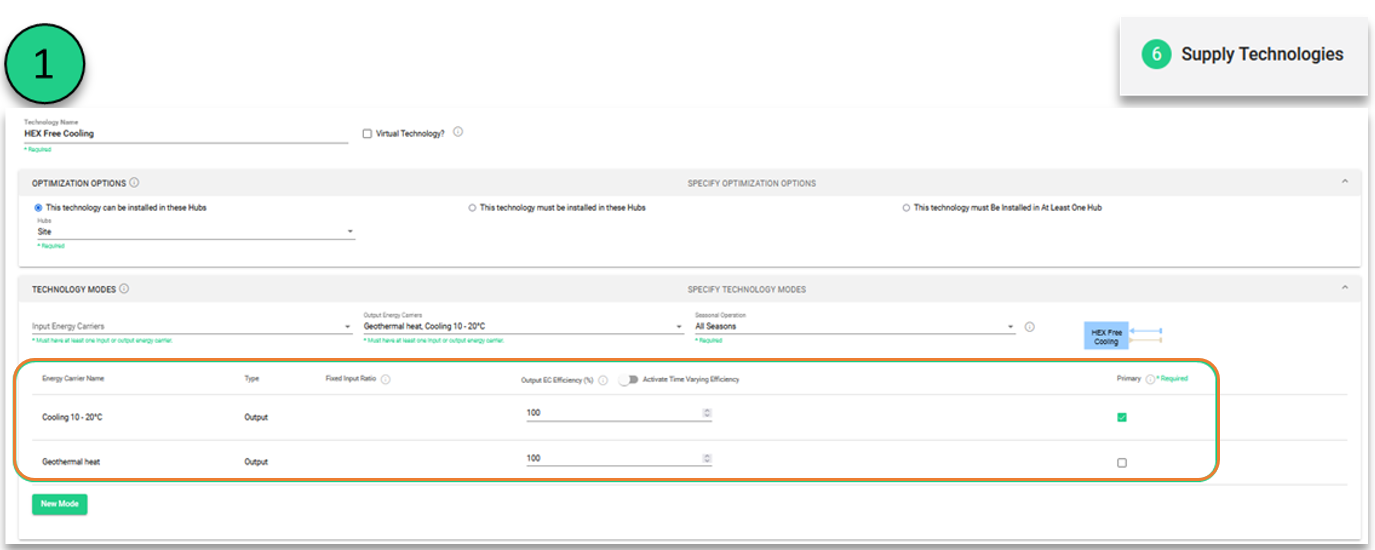
Figure 51 Modelling of a HEX for free cooling with geothermal storage
- Free Cooling (with cold water storage)
Two cases must be considered here:
A storage without charging and discharging losses
A storage with charging and discharging losses
- Storage without charging and discharging losses
For a storage without charging and discharging losses (= charging / discharging efficiencies of 100%), it is straight forward:
Make sure that the charging and discharging efficiencies are equal to 100%
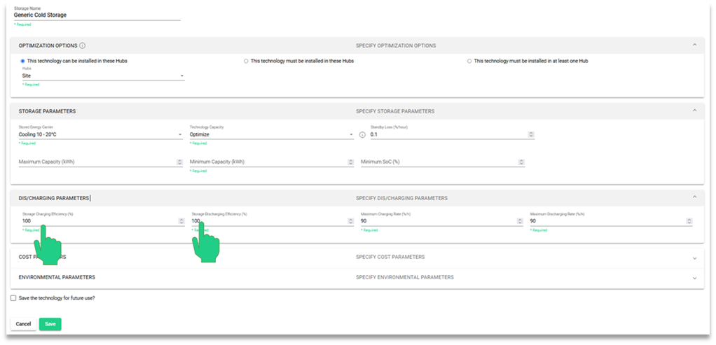
Figure 52 Charging and discharging parameters for a generic cold storage for free cooling
- Storage with charging and discharging losses
As the storage technology has the possibility to charge and discharge at the same time, this may result in losses. When set up incorrectly, the system can use this to destroy energy (by charging and discharging high quantities of energy). This behaviour is observed when it is profitable for a system to destroy energy, which is the case when free cooling is be used (and when the cost and CO2 emissions of operating the free cooling is lower than using the other systems, which is the idea of the free cooling). In this case, the storage must be possible only for the actively chilled water.
Set-up summary
Energy Carriers | Energy Demands | Imports | Exports |
| Supply technology |
| |||||
Brine water | Brine water HP 2 | Brine water HP 3 | HEX waste heat to geothermal | HEX Free cooling | Generic Borehole | Virtual technology | |||||
Electricity |
| X |
| Primary Input | (primary) Input | Primary Input |
|
|
|
| |
Geothermal heat |
|
|
| Input |
|
| (primary) output | Output | X |
| |
Ambient heat |
| X |
|
| Input |
|
|
|
|
| |
Heat 30-40°C | X |
|
| (primary) | (primary) Output |
|
|
|
|
| |
Cooling 10-20°C | X |
|
|
|
|
|
| (primary) output |
| (primary) output | |
Active Cooling |
|
|
|
|
| (primary) output |
|
|
| (primary) input | |
Waste heat |
|
| X |
|
| Output | (primary) input |
|
|
| |
Set-up implementation
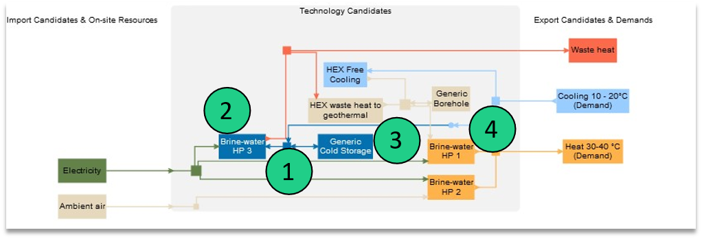
Figure 53 Set-up implementation of free cooling with a cold water storage
In this case, the cooling must be separated into two energy carriers: (e.g.) Cooling and active cooling. This is done so that the cooling production and storage use another energy carrier (active cooling) than the energy carrier produced by the HEX Free cooling (cooling 10-20°C), which has for effect, that the cooling 10-20°C cannot be stored within the cold storage.
The following model is based on the free cooling without storage model (section 5.1.1.2)
From there on, the custom cooling energy carrier ‘active cooling’ must first be added to the energy carriers.
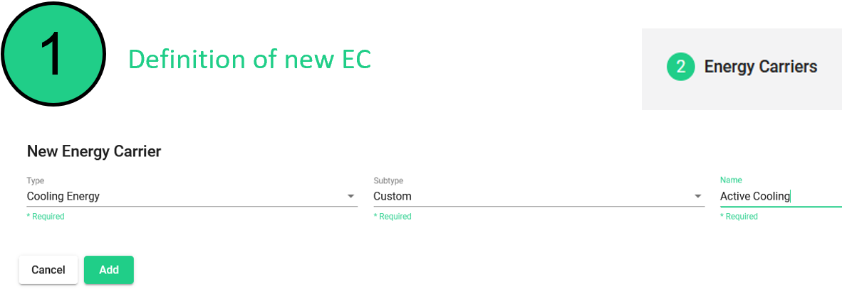
Figure 54 Definition of Cooling Energy as an energy carrier to use for free cooling with cold water storage
Under the tab supply technologies, the output of the mode 3 of the brine water heat pump is changed to ‘active cooling’.
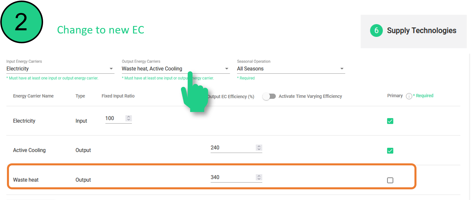
Figure 55 Change of output energy carrier to active cooling for cold water storage
The generic storage can be added, as a storage for active cooling.
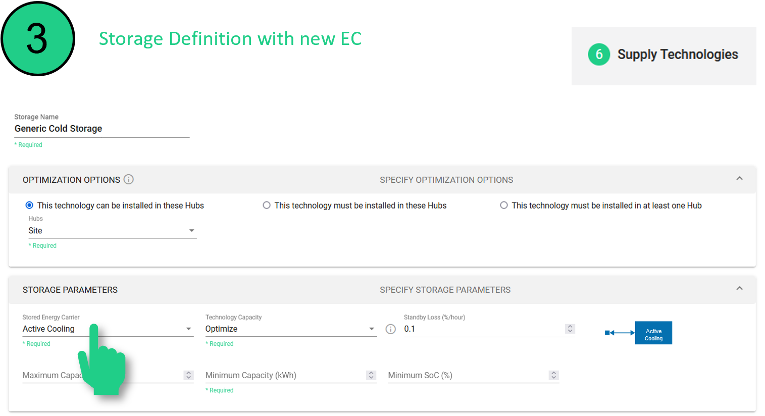
Figure 56 Storage Definition of a generic cold storage using to use in active cooling
Finally, to allow for the system to cover the cooling demand with the active cooling, a virtual technology is added, transforming active cooling into cooling 10-20°C (the energy carrier of the demand).
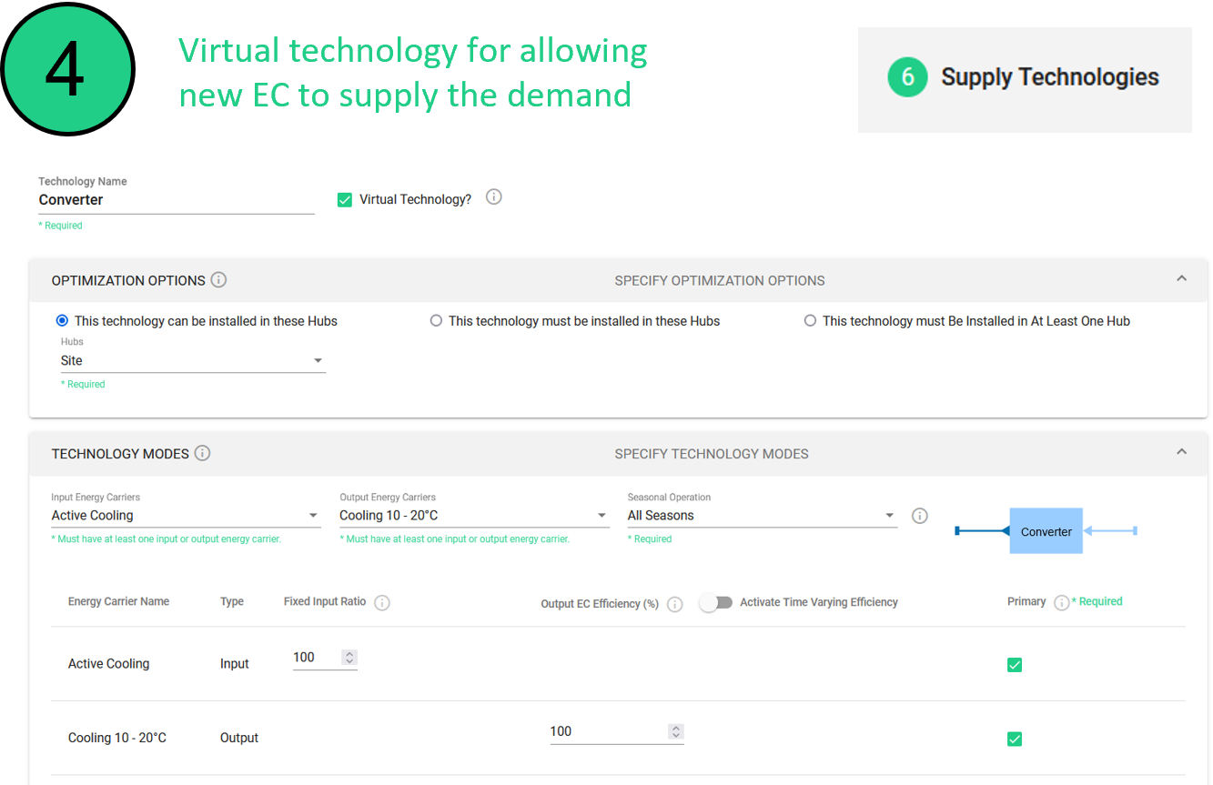
Figure 57 Definition of a virtual technology to convert active cooling into cooling energy
- Free Cooling as export
Finally, there are some cases where free cooling is to be used as a 'bonus', meaning that the tenants won't have guarantee that their building is cooled. In this case, this 'bonus' must be modelled as an export rather than a demand. Indeed, modelling it as a demand would force its production. The system is simple: a brine water heat pump can work on a geothermal borehole. To regenerate this borehole, free cooling of the buildings can be used (reminder: a borehole modelled as a storage need to be charged and discharged).
Set-up implementation
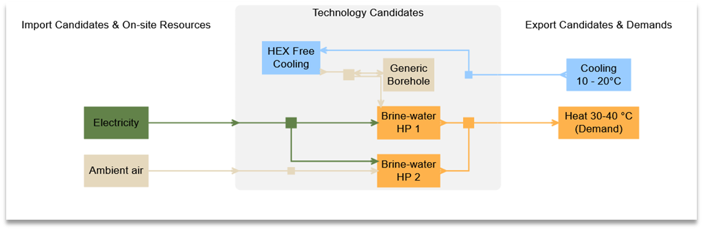
Figure 58 System diagram including free cooling as an export
Set-up summary
Energy Carriers | Energy Demands | Imports | Exports |
| Supply technology | Storage technology | ||
Brine water HP 1 | Brine water HP 2 | HEX Free cooling | Generic borehole | |||||
Electricity |
| X |
| Primary Input | Primary Input |
| X | |
Geothermal heat |
|
|
| Input |
| Output |
| |
Ambient heat |
| X |
|
| Input |
|
| |
Heat 30-40°C | X |
|
| (primary) Output | (primary) Output |
|
| |
Cooling 10-20°C | X |
|
|
|
| (primary) output |
| |
Set-up implementation
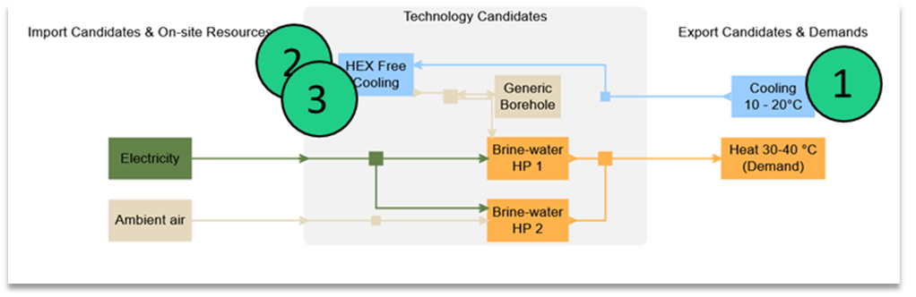
Figure 59 Set-up implementation of a system using free cooling as an export
First, the energy carrier for the free cooling must be added (in this case Cooling 10-20°C)
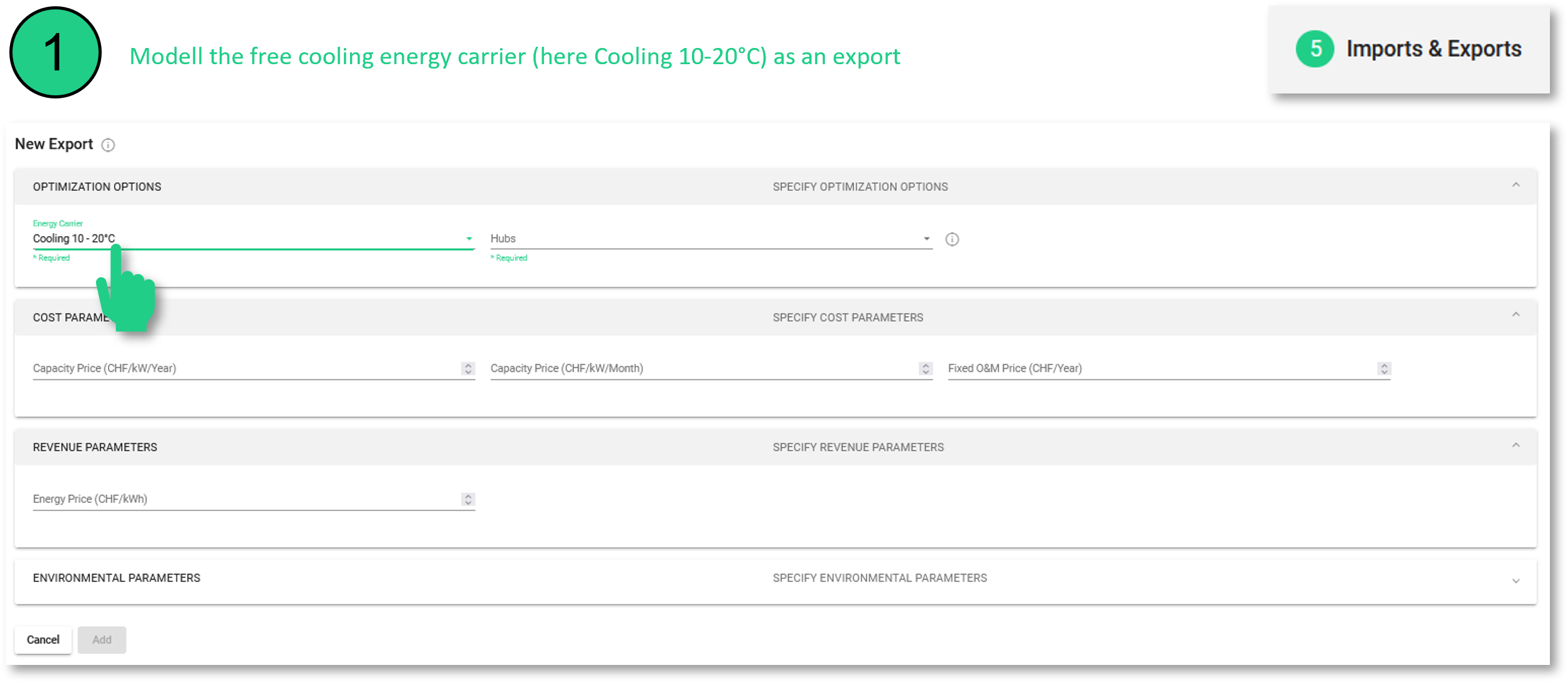
Figure 60 Modelling of free cooling as an energy carrier as an export
The capacity of the free cooling heat exchanger must be limited to avoid infinite production of (very cheap) low temperature heat.
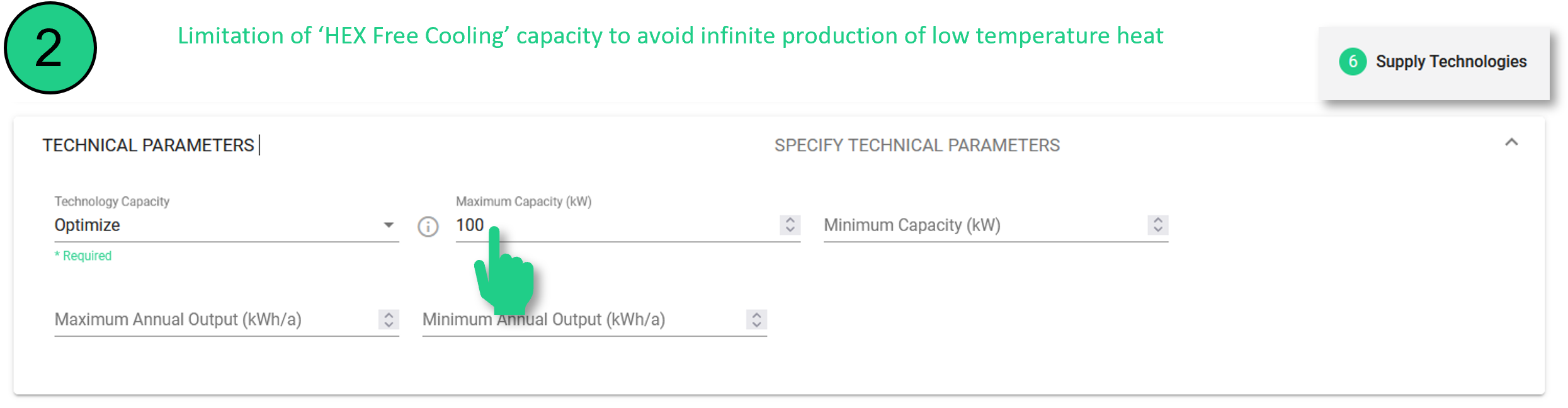
Figure 61 Limitation of the HEX free cooling capacity to avoid the infinite production of low temperature heat
Monthly time varying efficiencies can be used to further modulate this capacity for every month (by setting efficiencies lower than 100%). This must be done for both outputs.
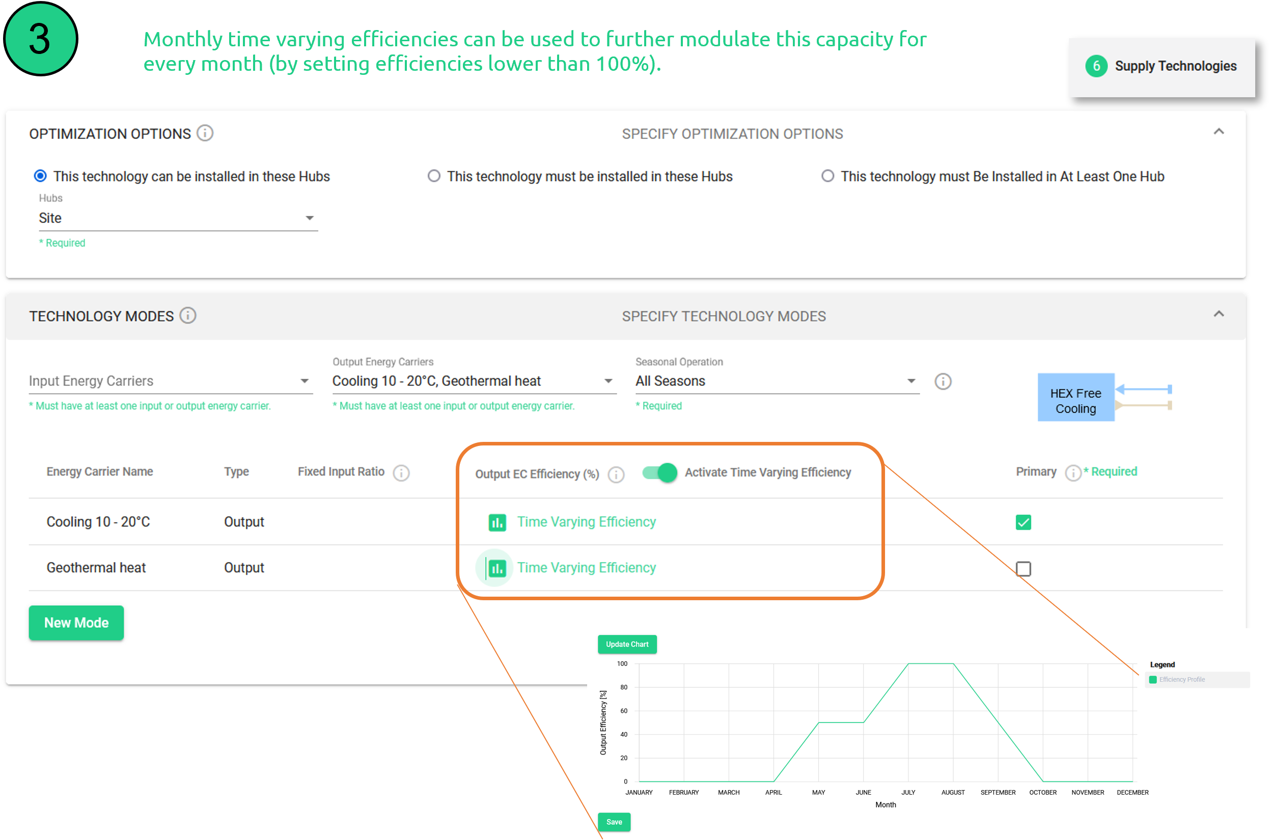
Figure 62 addition of a time varying efficiency to modulate the capacity of a HEX